Protein Features and Neural Networks

This is Preliminary Note 2 for the Protein & Artificial Intelligence course (Spring 2026), co-taught by Prof. Sungsoo Ahn and Prof. Homin Kim at KAIST. It builds on Preliminary Note 1 (Introduction to Machine Learning with Linear Regression). Now that you know what tensors and gradients are, this note answers two questions: how do you turn protein data into numerical features that a neural network can process, and what neural network architectures learn useful representations from those features?

Introduction

A neural network cannot process amino acid sequences stored in text files. Bridging from raw biological data to trained predictors requires three things: a way to read the standard sequence file format (FASTA), a way to encode sequences as numerical features and pass them through neural network architectures, and a way to formulate different biological questions as the right mathematical task.

Features are the numerical inputs you construct from raw data — one-hot encodings, amino acid compositions, and the like. Representations are the internal vectors that a neural network learns in its hidden layers. Features are hand-crafted; representations are learned.

Roadmap

Prerequisites

Tensors, gradient descent, and the learning cycle (model, loss, gradients, update) from Preliminary Note 1.

1. Protein Sequences and FASTA

Every protein ML pipeline starts with sequence data, and sequence data lives in FASTA files.

1.1 FASTA: The Universal Sequence Format

FASTA is the simplest bioinformatics file format. Each entry consists of a header line starting with >, followed by one or more lines of amino acid sequence:

>sp|P0A6Y8|DNAK_ECOLI Chaperone protein DnaK
MGKIIGIDLGTTNSCVAIMDGTTPRVLENAEGDRTTPSIIAYTQDGETLVGQPAKRQAVT
NPQNTLFAIKRLIGRRFQDEEVQRDVSIMPFKIIAADNGDAWVEVKGQKMAPPQISAEVL

The header in this example follows UniProt¹ conventions. sp indicates Swiss-Prot (the manually curated portion of UniProt). P0A6Y8 is the accession number — a unique identifier for this protein. DNAK_ECOLI is the entry name. Different databases use different header conventions, so always check the source before writing a parser.

1.2 Parsing FASTA with Biopython

Biopython is the standard library for biological file parsing in Python. A few lines of code are enough to load every sequence from a FASTA file into a dictionary keyed by accession:

from Bio import SeqIO

def load_fasta(filepath):
    """Load all sequences from a FASTA file into a dictionary."""
    sequences = {}
    for record in SeqIO.parse(filepath, "fasta"):
        sequences[record.id] = str(record.seq)
    return sequences

# Example usage
seqs = load_fasta("proteins.fasta")
for name, seq in list(seqs.items())[:3]:
    print(f"{name}: {len(seq)} residues, starts with {seq[:10]}...")

Good parsers read records lazily — one at a time — rather than loading the entire file into memory. This matters when processing databases with millions of entries.

2. From Protein Features to Neural Networks

The 20 standard amino acids. Amino acids are grouped by their side-chain chemistry: nonpolar/hydrophobic (red), polar uncharged (blue), positively charged (green), and negatively charged (orange). Bar heights show approximate molecular weights. These chemical differences determine how each amino acid contributes to protein folding and function.

The amino acid sequence is the primary structure of a protein — the linear chain of residues² encoded by the gene.

To feed a protein into a neural network, we must convert its sequence into numerical features, then build an architecture that can learn from those features.

2.1 One-Hot Encoding

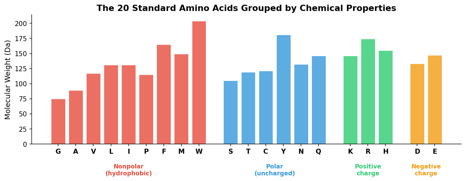
The most straightforward feature is a one-hot encoding³. In NLP, a vocabulary of 50,000 words maps each word to a one-hot vector of length 50,000 — enormously sparse, which is why language models compress these into dense embeddings. Protein sequences face the same encoding problem on a smaller scale: 20 amino acids rather than 50,000 words. Each amino acid at position \(i\) becomes a binary vector of length 20, with a single 1 indicating which residue is present:

A full protein of length \(L\) becomes a feature matrix \(\mathbf{X} \in \mathbb{R}^{L \times 20}\).

import torch

AMINO_ACIDS = "ACDEFGHIKLMNPQRSTVWY"
aa_to_idx = {aa: i for i, aa in enumerate(AMINO_ACIDS)}

def one_hot_encode(sequence: str) -> torch.Tensor:
    """One-hot encode a protein sequence as a PyTorch tensor."""
    encoding = torch.zeros(len(sequence), 20)
    for i, aa in enumerate(sequence):
        if aa in aa_to_idx:
            encoding[i, aa_to_idx[aa]] = 1.0
    return encoding

# Example: encode the first 5 residues of hemoglobin alpha
enc = one_hot_encode("MVLSP")
print(enc.shape)  # torch.Size([5, 20])

One-hot encoding preserves the full sequence — every position and every residue identity. Its limitation is that it treats every amino acid as equally different from every other. Learned embeddings (covered in the main lectures) address this by replacing each one-hot vector with a trainable continuous vector.

2.2 From Features to PyTorch Tensors

A neural network does not process one protein at a time. Training requires batches — groups of proteins processed together for computational efficiency. But proteins have different lengths, so we must pad every sequence to a common length before stacking them into a tensor. NLP pipelines face the same challenge: sentences in a batch range from 3 to 50 tokens, so shorter sentences are padded with a special [PAD] token to match the longest. Protein sequences require identical treatment.

After one-hot encoding, each protein of length \(L\) is a matrix of shape \((L, 20)\). We choose a fixed maximum length \(L_{\max}\), pad shorter proteins with zero vectors, and truncate longer ones. Stacking \(B\) proteins gives a 3D tensor of shape \((B, L_{\max}, 20)\). For an MLP, which expects a flat vector as input, we flatten each protein’s matrix into a single vector of dimension \(L_{\max} \times 20\).

from torch.utils.data import TensorDataset, DataLoader

# Suppose we have protein sequences and their solubility labels
sequences = ["MGKIIGIDLG...", "MSKGEELFTG...", "MVLSPADKTN..."]
labels = [1, 1, 0]  # 1 = soluble, 0 = insoluble

# One-hot encode and pad to a fixed maximum length
max_len = 100  # Truncate longer proteins, pad shorter ones with zeros
features = torch.zeros(len(sequences), max_len, 20)
for i, seq in enumerate(sequences):
    L = min(len(seq), max_len)
    features[i, :L] = one_hot_encode(seq[:L])
labels = torch.tensor(labels, dtype=torch.long)

print(features.shape)  # torch.Size([3, 100, 20]) — 3 proteins, padded

# Flatten each protein's matrix into a single vector for the MLP
features_flat = features.view(len(sequences), -1)
print(features_flat.shape)  # torch.Size([3, 2000]) — ready for MLP input

# Wrap in a dataset and data loader
dataset = TensorDataset(features_flat, labels)
loader = DataLoader(dataset, batch_size=32, shuffle=True)

# Training loop iterates over batches
for batch_features, batch_labels in loader:
    # batch_features shape: (batch_size, 2000)
    # batch_labels shape:   (batch_size,)
    pass  # feed to neural network

A data loader handles shuffling, batching, and iterating: each iteration yields a batch of flattened feature vectors and their corresponding labels, ready to be passed through a neural network. Note that flattening discards the sequential structure — the MLP treats position 1 and position 100 as unrelated inputs. The main lectures introduce architectures (CNNs, transformers) that exploit this sequential ordering.

2.3 Why Linear Models Are Not Enough

A feature vector is not a prediction. To go from a one-hot encoded sequence to a solubility score, we need a function — and a linear model \(\hat{y} = \mathbf{W}\mathbf{x} + b\) is limited to straight-line relationships.

A linear classifier can only draw flat decision boundaries — it cannot learn that a cluster of dark pixels in the center of an image means “pupil” while scattered dark pixels mean nothing. The same limitation appears in proteins: solubility depends on nonlinear combinations of features — a cluster of five hydrophobic residues in a row is a strong signal for a transmembrane helix (likely insoluble), while the same five residues scattered throughout the sequence may have no effect. A linear model treats both cases identically.

Stacking two linear layers does not help:

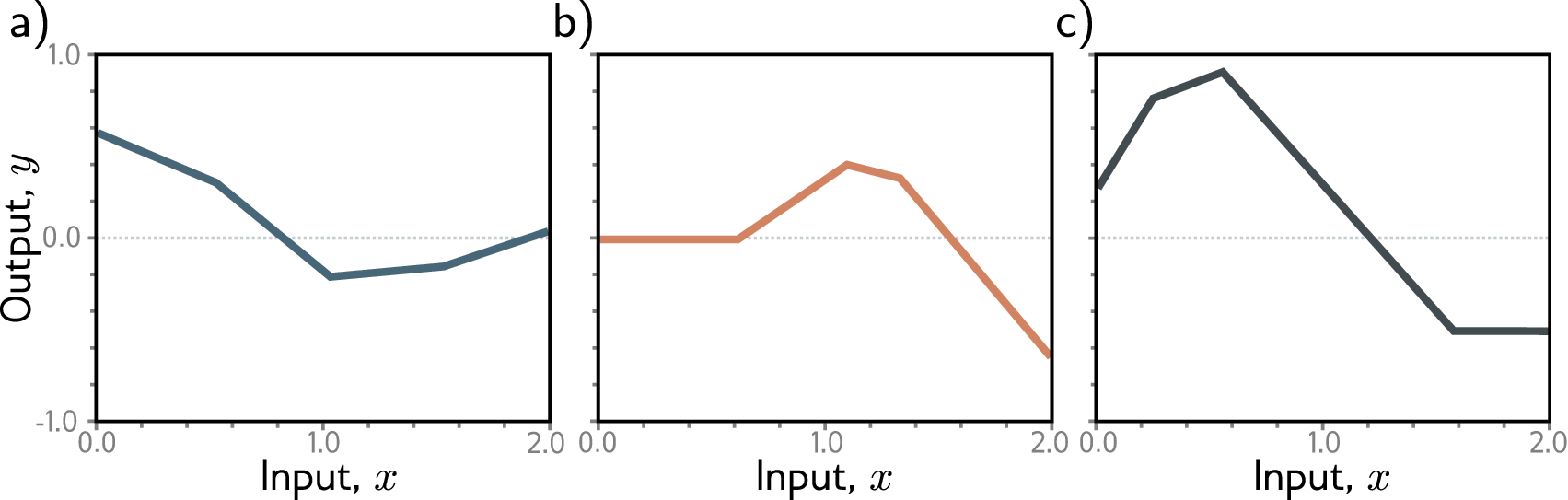
The composition of two linear transformations is still a single linear transformation. No matter how many linear layers we stack, the result collapses to one matrix multiplication — we gain no expressive power. Breaking out of this collapse requires a nonlinear activation function between layers, which is exactly what a neural network provides.

2.4 The Single Neuron

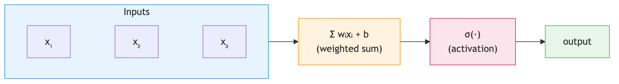
The artificial neuron takes multiple input features, computes a weighted sum, adds a bias, and applies a nonlinear function:

For protein solubility prediction, the input features \(x_1, x_2, \ldots, x_n\) are numerical values derived from the protein sequence. The weights \(w_1, w_2, \ldots, w_n\) determine how much each feature contributes to the solubility score. The bias \(b\) shifts the decision boundary, and the function \(\sigma\) — the activation function — introduces nonlinearity, allowing the neuron to model relationships that are not straight lines.

In vector notation, writing \(\mathbf{x} \in \mathbb{R}^n\) for the input and \(\mathbf{w} \in \mathbb{R}^n\) for the weight vector, and choosing \(\sigma\) as the sigmoid function, the single neuron computes:

This is exactly logistic regression — the classification analogue of the linear regression we saw in Preliminary Note 1. The neuron’s output is a probability, and the decision boundary is the set of points where \(\mathbf{w}^T \mathbf{x} + b = 0\) (i.e., where the output probability is exactly 0.5). In 2D feature space, this boundary is a line; in the high-dimensional space of our flattened sequence features, it is a hyperplane. Points on one side are classified as soluble, points on the other as insoluble.

A single neuron can only learn linear decision boundaries. This is sufficient for linearly separable problems but fails when the boundary between classes is curved or disconnected — which is why we need multiple layers.

2.5 Layers: Many Neurons in Parallel

Anatomy of a shallow neural network. (a) Full notation: input \(x\) is multiplied by input-to-hidden weights \(\theta_{ij}\) (our \(\mathbf{W}\)) and offset by biases \(\theta_{i0}\) (our \(\mathbf{b}\)), passed through hidden units \(h_1, h_2, h_3\) with ReLU activations (cyan diagonal lines), then combined with hidden-to-output weights \(\phi_i\) to produce output \(y\). The circled 1's represent bias inputs. (b) Simplified diagram omitting weight labels. Source: Prince, Understanding Deep Learning, Fig 3.1 (CC BY-NC-ND).

A fully connected network with one hidden layer. Four input features \(x_1, \ldots, x_4\) each connect to all five hidden units \(h_1, \ldots, h_5\) (every arrow is a learned weight). The hidden layer applies a nonlinear activation, then connects to three outputs \(o_1, o_2, o_3\). "Fully connected" means every unit in one layer connects to every unit in the next. This is the \(\mathbf{h} = \sigma(\mathbf{W}\mathbf{x} + \mathbf{b})\) from the text. Source: Zhang et al., Dive into Deep Learning, Fig 5.1.1 (CC BY-SA 4.0).

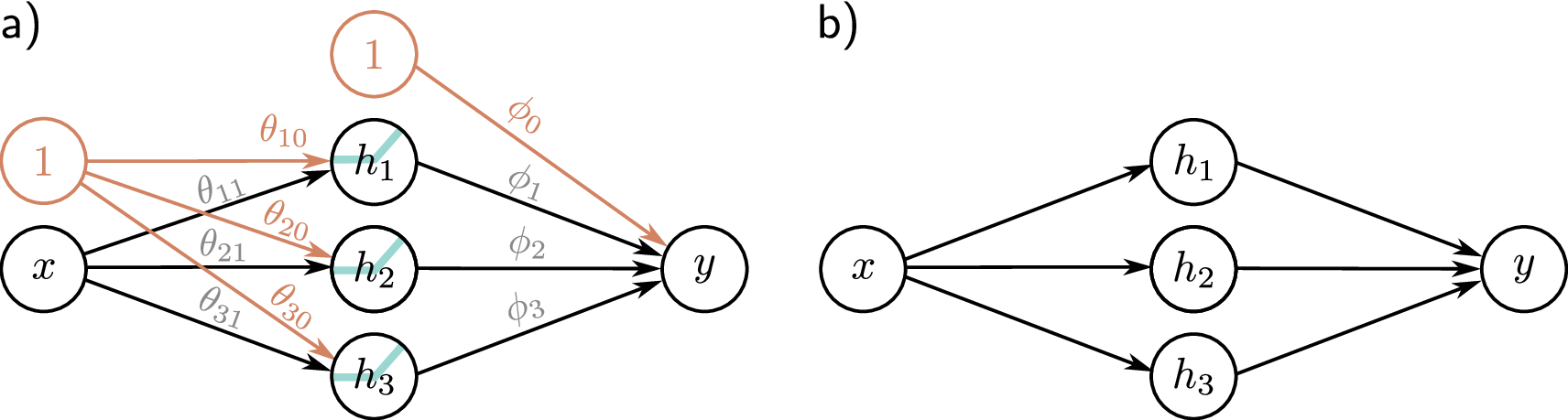
Arrange many neurons in parallel — each receiving the same input features but with different weights — and you get a layer. In computer vision, a fully connected layer might take a flattened 224x224x3 image (150,528 dimensions) and compress it to 512 hidden units. For protein sequences, the dimensions are smaller but the architecture is identical. With 64 neurons processing a \(d\)-dimensional input, you get a 64-dimensional representation — 64 different weighted combinations of the input features. This can be written compactly as a matrix equation:

Tracing the dimensions explicitly:

Each row of \(\mathbf{W}\) is one neuron’s weight vector. Row \(k\) computes the dot product⁴ \(\mathbf{w}_k^T \mathbf{x} + b_k\), producing one scalar.

This is a fully connected layer (also called a dense layer or linear layer). The total number of parameters is \(64d + 64\) (weights plus biases). For our padded protein sequences with \(d = L_{\max} \times 20 = 2{,}000\), that is already \(128{,}064\) parameters in a single layer. The nonlinear function \(\sigma\) applied after each layer is the activation function — Section 2.7 covers the main choices in detail. The most common default is ReLU: \(\text{ReLU}(z) = \max(0, z)\).

What a single hidden layer can compute. Three examples of piecewise-linear functions (input \(x\) → output \(y\)) produced by a shallow network with ReLU activations. Each panel uses different weights and biases, yielding a different nonlinear mapping — none of which a linear model could represent. Source: Prince, Understanding Deep Learning, Fig 3.3 (CC BY-NC-ND).

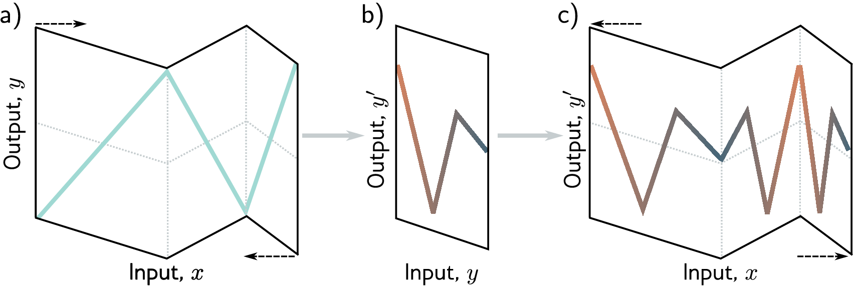
2.6 Why Depth Matters: The Power of Composition

A two-hidden-layer MLP for solubility prediction. The flattened padded sequence is transformed through two hidden layers of decreasing width (64, 32), each applying a linear transformation followed by an activation function. The output layer produces two scores (soluble vs. insoluble).

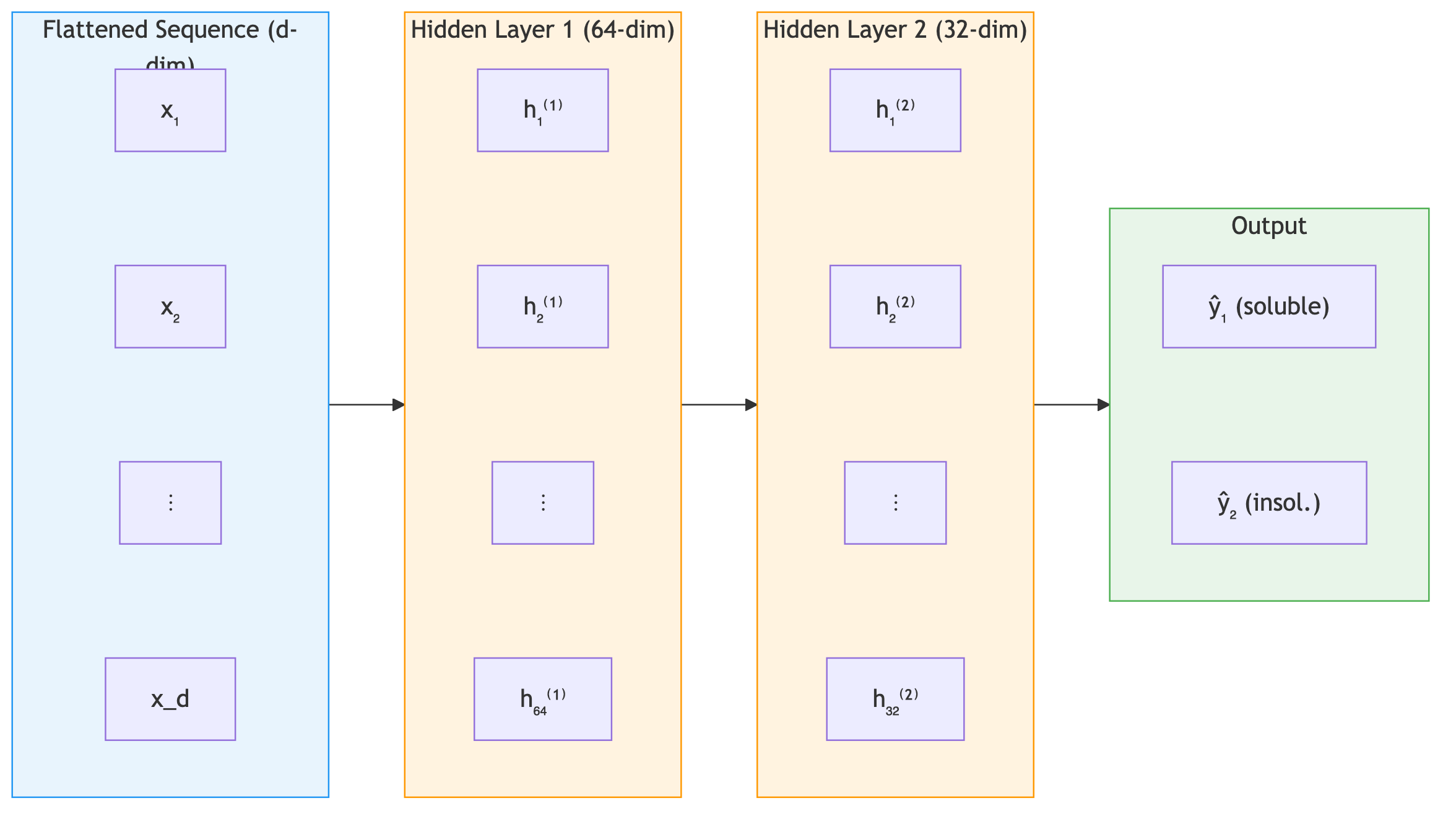
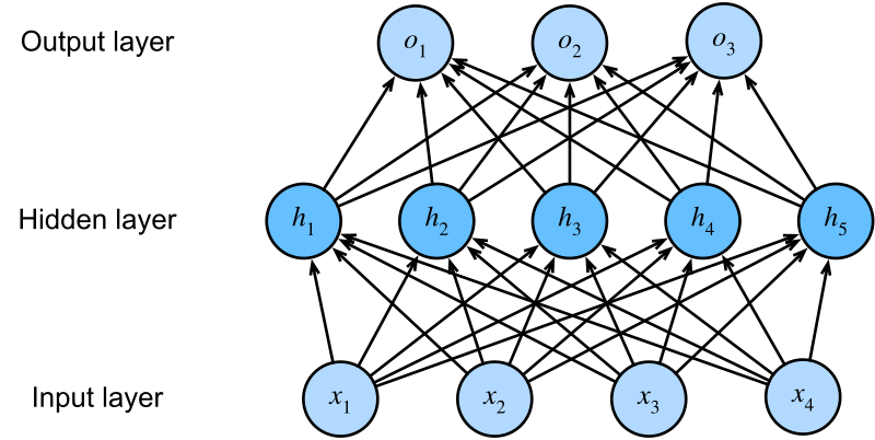
The power of neural networks comes from stacking multiple layers. An \(n\)-layer network, called a multi-layer perceptron (MLP), composes \(n\) transformations:

Here \(\mathbf{W}_l \in \mathbb{R}^{d_l \times d_{l-1}}\) maps from the \((l{-}1)\)-th layer’s width \(d_{l-1}\) to the \(l\)-th layer’s width \(d_l\), with \(\mathbf{b}_l \in \mathbb{R}^{d_l}\) and \(\mathbf{h}_l \in \mathbb{R}^{d_l}\) (taking \(d_0\) as the input dimension and \(\mathbf{h}_0 = \mathbf{x}\)). Each hidden layer takes the previous layer’s output \(\mathbf{h}_{l-1}\) as input, applies a linear transformation followed by a nonlinear activation, and produces a new representation \(\mathbf{h}_l\). The final layer typically has no activation (for regression) or a sigmoid/softmax (for classification). Deeper networks can represent complex functions efficiently because each layer builds more abstract features from the previous layer’s output.

Deep networks build hierarchical representations. In image recognition, early layers detect edges, middle layers combine edges into textures and shapes, and final layers recognize objects. In NLP, early layers capture character patterns, middle layers capture word meanings, and final layers capture sentence-level semantics. Protein networks follow the same principle. For a protein solubility predictor, the first layer detects which positions and amino acid identities are informative, extracting basic patterns from the flattened sequence. The second layer combines these into higher-level patterns — local composition trends, position-specific signals — and the output layer maps those abstract representations to a solubility prediction.

Why depth is powerful: function composition. (a) The first layer computes a piecewise-linear function \(y = f_1(x)\) (black), folding the input space at each kink (cyan shows the fold lines). (b) The second layer computes another piecewise-linear function \(y' = f_2(y)\) in the transformed space. (c) The composition \(y' = f_2(f_1(x))\) produces a function with far more linear regions than either layer alone — each fold in (a) multiplies the complexity of (b). A shallow network of the same width could not produce this many distinct regions. Source: Prince, Understanding Deep Learning, Fig 4.4 (CC BY-NC-ND).

In practice, deeper networks are not always better. Very deep networks can be harder to train (gradients may vanish or explode as they propagate through many layers). Techniques like residual connections, normalization layers, and careful initialization have made training deep networks practical.

2.7 Activation Functions

Without the activation function \(\sigma\) applied element-wise after each linear transformation, stacking layers collapses to a single linear transformation (Section 2.3). Activation functions are what give neural networks their expressive power.

Common activation functions. Each panel plots the activation \(\text{a}[z]\) (our \(\sigma(z)\)) as a function of its pre-activation input \(z\). (a) Sigmoid squashes to \((0, 1)\); tanh squashes to \((-1, 1)\). (b) Leaky ReLU and PReLU pass a small slope for negative inputs, avoiding "dead neurons." (c) Smooth variants used in modern architectures: softplus, GeLU (used in protein language models), SiLU. (d–f) More specialized activations including ELU, SELU, and Swish. Source: Prince, Understanding Deep Learning, Fig 3.13 (CC BY-NC-ND).

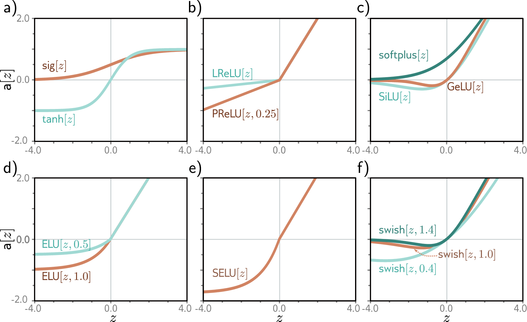
ReLU (\(\text{ReLU}(z) = \max(0, z)\)) is the default for hidden layers: it zeros out negative values, passes positive values unchanged, and is fast to compute, though neurons stuck at zero (“dead neurons”) stop learning entirely. GELU is a smooth variant of ReLU used in transformer models including protein language models like ESM, offering slightly better training dynamics. For output layers, sigmoid (\(\sigma(z) = 1/(1 + e^{-z})\)) squashes a scalar to \((0, 1)\) for binary classification, while softmax normalizes a vector into a probability distribution for multi-class classification.

2.8 nn.Module: PyTorch’s Building Block

Every PyTorch neural network inherits from nn.Module, which handles parameter tracking, GPU transfer, and model saving. A custom network specifies two things: what layers exist (__init__), and how data flows through them (forward).

import torch
import torch.nn as nn

class SolubilityPredictor(nn.Module):
    """A feedforward network for protein solubility prediction."""

    def __init__(self, input_dim, hidden_dim, output_dim):
        super().__init__()
        # First fully connected layer: input features → hidden representation
        self.fc1 = nn.Linear(input_dim, hidden_dim)
        # Activation function
        self.relu = nn.ReLU()
        # Second fully connected layer: hidden representation → prediction
        self.fc2 = nn.Linear(hidden_dim, output_dim)

    def forward(self, x):
        # x shape: (batch_size, input_dim)
        h = self.fc1(x)    # Features → hidden representation
        h = self.relu(h)   # Nonlinear activation
        out = self.fc2(h)  # Representation → prediction
        return out

# Flattened padded sequences: max_len=100 × 20 amino acids = 2000-dim input
model = SolubilityPredictor(input_dim=2000, hidden_dim=64, output_dim=2)

# Pass a batch of 32 proteins through the model
features = torch.randn(32, 2000)  # 32 proteins, flattened padded sequences
predictions = model(features)    # Shape: (32, 2) — scores for [soluble, insoluble]
print(predictions.shape)

The data flow follows the pattern from Section 2.5: input features pass through a linear layer and activation to produce a hidden representation, then a second linear layer maps that representation to a prediction. PyTorch handles the backward pass (gradient computation) automatically — you only specify the forward computation.

2.9 Common Layer Types

The building blocks of protein AI models: linear layers, activations, normalization, dropout, and embeddings.

# --- Linear layer ---
# Computes y = Wx + b. The fundamental building block.
nn.Linear(in_features=20, out_features=64)

# --- Activation functions ---
nn.ReLU()        # max(0, x) — simple, effective, the default choice
nn.GELU()        # Smooth approximation of ReLU, used in transformer models
nn.Sigmoid()     # Squashes output to (0, 1), useful for binary probabilities
nn.Softmax(dim=-1)  # Normalizes a vector to sum to 1 (probability distribution)

# --- Normalization layers ---
# Stabilize training by normalizing intermediate activations
nn.LayerNorm(normalized_shape=64)    # Normalizes across features (used in transformers)
nn.BatchNorm1d(num_features=64)      # Normalizes across the batch dimension

# --- Dropout ---
# Randomly zeros out neurons during training to prevent overfitting
nn.Dropout(p=0.1)  # Each neuron has a 10% chance of being turned off per forward pass

# --- Embedding layer ---
# Maps discrete tokens (like amino acid indices) to continuous vectors
# 21 possible tokens (20 amino acids + 1 padding), each mapped to a 64-dim vector
nn.Embedding(num_embeddings=21, embedding_dim=64)

3. Task Formulations

The first design decision in any protein ML project: what type of output does the model produce? This choice determines the output activation, loss function, and evaluation metrics.

Regression predicts a continuous number (melting temperature, binding affinity) with MSE loss. Binary classification outputs a probability via sigmoid and applies a threshold. Multi-class classification extends this to \(C\) categories via softmax. Multi-label classification treats each label independently — a protein can be both kinase and membrane-bound. Sequence-to-sequence produces one output per residue, as in secondary structure prediction (helix/sheet/coil at each position).

Key Takeaways

1. FASTA is the standard format for protein sequences. Biopython handles parsing. Loading and encoding sequences is the entry point to any protein ML pipeline.

2. Features are hand-crafted numerical inputs: one-hot encoding converts each amino acid into a binary vector, preserving the full sequence. Features are padded, flattened, and converted to PyTorch tensors for training.

3. Neural networks are compositions of simple layers: linear transformations followed by nonlinear activations. Depth enables hierarchical representation learning — each layer builds more abstract representations from the previous layer’s output.

4. Task formulations map biological questions to mathematical outputs: regression for continuous values, classification for categories, sequence-to-sequence for per-residue predictions.

5. Next up: Preliminary Note 3 puts these features and architectures to work in a complete training pipeline — loss functions, optimizers, and validation.