Introduction to Machine Learning with Linear Regression
This is Preliminary Note 1 for the Protein & Artificial Intelligence course (Spring 2026), co-taught by Prof. Sungsoo Ahn and Prof. Homin Kim at KAIST. It is designed as a self-study resource: biology-background students should be able to work through it independently before the first in-class lecture. This note assumes basic Python fluency and comfort with linear algebra.
Introduction
Imagine you have cloned a gene, designed a construct, and transformed E. coli cells. After overnight expression you lyse the cells, spin down the debris, and pipette off the soluble fraction — only to find that your target protein is trapped in insoluble inclusion bodies. You have just wasted days of bench time. Now imagine a computer program that, given nothing but the amino acid sequence of your construct, predicts with high accuracy whether the protein will be soluble. Building that program is a machine learning problem, and understanding how to solve it is the goal of this note and the next three.
By the end of these four notes, you will have a working solubility predictor — a model that takes an amino acid sequence and outputs a probability. This first note builds the foundation: what machine learning actually is, how data becomes tensors, and how a model learns from a single gradient step.
Roadmap
| Section | Topic | Why You Need It |
|---|---|---|
| 1 | What Is Machine Learning? | The foundational concepts: function approximation and generalization |
| 2 | The Machine Learning Pipeline | The big picture: how raw protein data becomes a trained model |
| 3 | PyTorch Tensors | Tensors are the data structure that stores every protein feature, every weight, and every gradient |
| 4 | Linear Regression: A First Model | Building a first model, measuring its mistakes, and using gradients to improve it |
Prerequisites
This note assumes basic Python fluency and comfort with linear algebra: vectors, matrices, and matrix multiplication. If the expression \(\mathbf{y} = \mathbf{W}\mathbf{x} + \mathbf{b}\) looks unfamiliar, review the linear algebra appendix in Goodfellow et al. [a] before continuing.
1. What Is Machine Learning?
Learning as Function Approximation
Radiologists develop intuitions about which shadow on a CT scan signals a tumor; experienced editors can tell within a sentence whether a text was machine-generated. These intuitions are real but hard to articulate as explicit rules. The same is true in biochemistry: experienced biochemists know that highly charged proteins tend to be soluble and long hydrophobic stretches spell trouble, yet translating that knowledge into a precise algorithm is remarkably difficult.
Machine learning is function approximation: the systematic version of this pattern recognition. There exists some unknown function \(f^*\) that maps inputs to outputs. In protein science, this might mean mapping an amino acid sequence to a solubility label (soluble or insoluble). In a general setting, it might mean mapping a photograph of a person’s face to their age, or mapping a house’s features (square footage, location, number of rooms) to its sale price. In both cases, we cannot write down \(f^*\) explicitly because the relationship is too complex for any simple formula. Instead, we define a family of candidate functions \(f_\theta\), parameterized by adjustable numbers \(\theta\) (called parameters or weights), and we search for the particular values of \(\theta\) that make \(f_\theta\) approximate \(f^*\) as closely as possible.
This search is what “training” means. More precisely, this is an optimization problem. Given a training set \(\{(\mathbf{x}_i, y_i)\}_{i=1}^n\) of \(n\) input-output pairs, we define a loss function \(\mathcal{L}(\theta)\) that measures how poorly \(f_\theta\) fits the data (Section 4 makes this concrete). Training then amounts to solving:
\[\theta^* = \arg\min_\theta \mathcal{L}(\theta)\]In words: find the parameter values \(\theta^*\) that minimize the total prediction error over the training set. In practice, an optimization algorithm sees thousands of proteins with known properties and gradually adjusts \(\theta\) to reduce \(\mathcal{L}(\theta)\). The result is a function that captures the statistical regularities in the data — amino acid composition biases, charge distributions, hydrophobicity patterns — as numerical weights.
Generalization: The Real Goal
What matters is not training performance but generalization: accurate predictions on new proteins that were not part of the training data. An image classifier trained on 1,000 cat photos can memorize fur patterns and fail on cats in unusual poses; a protein model can memorize its training set and fail the moment it sees a novel sequence. Every technique in this course — model size, regularization, data splitting — exists to close the gap between training and test performance (formalized as the bias-variance tradeoff in Preliminary Note 3). The linear model we build in Section 4 illustrates one source of that gap: it can only learn straight-line relationships, yet real protein properties depend on nonlinear combinations of features — a cluster of five hydrophobic residues in a row matters far more than five scattered throughout the sequence. Preliminary Note 2 introduces neural networks, which overcome this limitation by composing simple nonlinear transformations into powerful function approximators.
2. The Machine Learning Pipeline
Every project follows the same arc.

You start with data — proteins and their labels, mined from databases like UniProt1 or high-throughput expression studies. The data is messy: ambiguous amino acid codes (B for Asp or Asn, X for unknown), sequences of wildly different lengths, inconsistent formats. You clean it, encode it as numerical features — one-hot vectors, physicochemical descriptors, learned embeddings (the subject of Preliminary Note 2) — and feed it to a model.
The model trains: it sees thousands of labeled proteins and adjusts its parameters to minimize prediction errors (Section 4 makes this concrete). Then you evaluate — and evaluation is trickier than it sounds. In computer vision, training and test images are typically split randomly — but even there, duplicate or near-duplicate images must be removed to prevent leakage. In NLP, temporal splits ensure the model never trains on future text. Protein data demands an even stricter protocol: related sequences often share properties, so a naive random train/test split lets the model “cheat” by recognizing near-duplicates. Proper evaluation requires sequence-identity-aware splitting2 to ensure the test set contains truly novel proteins (Preliminary Note 4 explains why this matters so much for solubility).
Finally, the model goes into production — where inference speed, memory constraints, and integration with laboratory workflows all matter.
3. PyTorch: Your Laboratory for Neural Networks
PyTorch [b] is the framework we use to build and train neural networks. It dominates deep learning research — ESM, OpenFold, and every major protein AI model is built on it. Code runs line by line (no deferred compilation), so debugging feels like debugging normal Python.
Tensors: The Atoms of Deep Learning
The core data structure in PyTorch is the tensor — a multi-dimensional array of numbers, like a NumPy array with superpowers. Tensors generalize scalars (0D), vectors (1D), and matrices (2D) to arbitrary dimensions. Images are stored as 4D tensors of shape (batch, channels, height, width) — a batch of 32 RGB images of size 224×224 has shape (32, 3, 224, 224). Text sequences become 3D tensors (batch, seq_len, embed_dim). Protein sequences follow the same pattern: a batch of protein sequences lives in a 3D tensor of shape (batch_size, sequence_length, features).

import torch

# From a Python list (e.g., hydrophobicity values for three amino acids)
x = torch.tensor([1.8, -4.5, 2.5])

# Random values from a standard normal distribution
x = torch.randn(3, 4)         # 3×4 matrix
print(x.shape)                 # torch.Size([3, 4])
print(x.dtype)                 # torch.float32
Tensors differ from NumPy arrays in two ways that matter: GPU acceleration and automatic differentiation.
Worked Example: Encoding a Protein Sequence as a Tensor
The pipeline mirrors NLP tokenization: a sentence like “The cat sat” is mapped to integer indices [2, 45, 91], then to dense vectors. For proteins, the vocabulary is the 20 standard amino acids. Trace the encoding of a short protein sequence through each stage, watching the tensor shape evolve.
import torch

# Our protein: the first 7 residues of human hemoglobin alpha chain
sequence = "MVLSPAD"

# Step 1: Map each amino acid to an integer index
# 20 standard amino acids → indices 1-20; 0 is reserved for padding
AA_TO_IDX = {aa: i + 1 for i, aa in enumerate("ACDEFGHIKLMNPQRSTVWY")}

indices = [AA_TO_IDX[aa] for aa in sequence]
print(f"Character sequence: {list(sequence)}")
print(f"Integer indices:    {indices}")
# Character sequence: ['M', 'V', 'L', 'S', 'P', 'A', 'D']
# Integer indices:    [11, 18, 10, 16, 13, 1, 3]

# As a tensor: shape (7,) — one integer per residue
seq_tensor = torch.tensor(indices)
print(f"Shape after integer encoding: {seq_tensor.shape}")  # torch.Size([7])

# Step 2: One-hot encode — each integer becomes a 20-dimensional binary vector
one_hot = torch.zeros(len(sequence), 20)
for i, idx in enumerate(indices):
    one_hot[i, idx - 1] = 1.0   # idx is 1-based, tensor indexing is 0-based

print(f"Shape after one-hot encoding: {one_hot.shape}")  # torch.Size([7, 20])
# Each row is all zeros except for a single 1 at the amino acid's position

# Step 3: Add a batch dimension (neural networks process batches of proteins)
batched = one_hot.unsqueeze(0)   # Add dim at position 0
print(f"Shape with batch dimension:   {batched.shape}")  # torch.Size([1, 7, 20])
# (batch_size=1, sequence_length=7, features=20)
The final shape (1, 7, 20) is the standard format for feeding protein sequences into neural networks: batch size, sequence length, and feature dimension. When processing 32 proteins at once, the shape becomes (32, max_len, 20) — Preliminary Note 2 covers how padding and flattening handle the fact that different proteins have different lengths.
The GPU Advantage
Neural networks are built from matrix multiplications, and GPUs accelerate these by computing thousands of independent dot products in parallel. In PyTorch, moving a tensor to the GPU is a single call (x.to('cuda')), and all tensors in an operation must live on the same device. Preliminary Note 3 covers the practical details when we write the training loop.
Tensor Operations
Tensors support all the arithmetic you would expect, with the same broadcasting rules3 as NumPy.
# Matrix multiplication (the workhorse of neural networks)
a = torch.randn(3, 4)
b = torch.randn(4, 5)
c = a @ b                # 3×4 times 4×5 → 3×5

# Broadcasting: a smaller tensor is "stretched" to match
a = torch.randn(3, 4)    # Shape: (3, 4)
b = torch.randn(4)       # Shape: (4,)
c = a + b                # b is added to each row → shape (3, 4)
4. From Data to Learning: A First Model
How does a model actually learn from data? The answer has four steps, which we build up one at a time using a concrete protein example:
- Define a model that makes predictions.
- Measure how wrong the predictions are with a loss function.
- Compute gradients that tell us how to adjust the model’s parameters to reduce the loss.
- Update the parameters and repeat.
A First Model: Linear Regression
Consider a concrete setup. In a classic regression problem, a model might predict house prices from features like square footage, number of rooms, and neighborhood — each feature gets a weight, the weighted sum plus a bias gives the prediction. The same structure applies to proteins: we have measured 10 physicochemical features for a single protein — molecular weight, isoelectric point, GRAVY score (hydrophobicity), instability index, and so on — and we want to predict its melting temperature. Call the true melting temperature \(y\) and our prediction \(\hat{y}\).
The simplest model is a weighted sum of the features plus a bias:
\[\hat{y} = w_1 \cdot x_{\text{MW}} + w_2 \cdot x_{\text{pI}} + w_3 \cdot x_{\text{GRAVY}} + \cdots + w_{10} \cdot x_{10} + b\]Here \(x_{\text{MW}}\) is the molecular weight, \(x_{\text{pI}}\) is the isoelectric point, and \(x_{\text{GRAVY}}\) is the hydrophobicity score. Each weight \(w_i\) controls how much one feature contributes to the prediction. A large positive \(w_3\) (the weight on GRAVY score) would mean more hydrophobic proteins are predicted to have higher melting temperatures. The bias \(b\) shifts the overall prediction up or down.
Using vector notation, we can write this more compactly. Let \(\mathbf{x} = [x_1, x_2, \ldots, x_{10}] \in \mathbb{R}^{10}\) be the feature vector for one protein, and \(\mathbf{w} = [w_1, w_2, \ldots, w_{10}] \in \mathbb{R}^{10}\) the weight vector. Then:
\[\hat{y} = \mathbf{x} \cdot \mathbf{w} + b = \sum_{j=1}^{10} x_j w_j + b\]
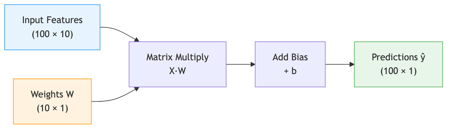
Now suppose we have not one protein but 100. We stack their feature vectors into a matrix \(\mathbf{X} \in \mathbb{R}^{100 \times 10}\), where each row is one protein’s features. A single matrix multiplication \(\mathbf{X}\mathbf{W}\) computes the weighted sum for all 100 proteins at once:
\[\hat{\mathbf{y}} = \mathbf{X}\mathbf{W} + b\]Here \(\mathbf{W} \in \mathbb{R}^{10 \times 1}\) is the weight vector reshaped as a column, and the result \(\hat{\mathbf{y}} \in \mathbb{R}^{100 \times 1}\) is a column of predictions — one per protein.
The following diagram illustrates this flow:
import torch

# Simulated data: 100 proteins, 10 physicochemical features each
# Each row of X is one protein's features: [mol. weight, pI, GRAVY, ...]
X = torch.randn(100, 10)   # 100 proteins × 10 features
y = torch.randn(100, 1) * 10 + 60   # True melting temperatures (centered ~60°C)

# Learnable parameters — requires_grad=True tells PyTorch to track gradients
W = torch.randn(10, 1, requires_grad=True)   # One weight per feature
b = torch.zeros(1, requires_grad=True)        # Bias term

# Forward pass: predict melting temperature for ALL 100 proteins at once
# X @ W computes the dot product of each protein's features with W
y_pred = X @ W + b              # Shape: (100, 1) — one prediction per protein
print(f"Predictions shape: {y_pred.shape}")  # torch.Size([100, 1])
\(\mathbf{W}\) and \(b\) are the learnable parameters, which we collectively denote as \(\theta = \{\mathbf{W}, b\}\). Different values of \(\theta\) give different predictions — and right now, with random weights, the predictions are terrible. The question is: how do we find better values?
Measuring Mistakes: The Loss Function
Our model makes predictions. How do we know how wrong they are?
We need a single number that summarizes the gap between predictions and reality. This number is called a loss function (sometimes called a cost function or objective function). For regression tasks like predicting melting temperature, a natural choice is the mean squared error (MSE):
\[\mathcal{L}_{\text{MSE}}(\theta) = \frac{1}{n}\sum_{i=1}^{n}(\hat{y}_i(\theta) - y_i)^2\]The predictions \(\hat{y}_i(\theta)\) depend on the current parameter values \(\theta\), so the loss itself is a function of \(\theta\). This computes the average squared difference between each prediction and the true value \(y_i\). Squaring serves two purposes: it makes all errors positive (an overestimate of +5°C and an underestimate of −5°C are equally bad), and it penalizes large errors disproportionately (an error of 10°C contributes 100 to the sum, while an error of 1°C contributes only 1).
# Loss: mean squared error (in units of °C²)
loss = ((y_pred - y) ** 2).mean()
print(f"Loss: {loss.item():.2f}")  # A single number measuring total prediction error
With a model and a loss function in hand, learning becomes an optimization problem: find the values of \(\theta\) that minimize \(\mathcal{L}(\theta)\). But how?
\(\mathcal{L}_{\text{MSE}}\) is one of many possible loss functions4. Preliminary Note 3 covers others suited to classification tasks.
Learning from Mistakes: Gradients and Optimization
We want to adjust \(\mathbf{W}\) and \(b\) to reduce the loss. The tool for this is the gradient — the vector of partial derivatives of the loss with respect to each parameter.
Deriving the Gradient for MSE
The gradient computation is straightforward. Consider a single weight \(w_j\). Recall that the prediction for one protein is \(\hat{y}_i = \sum_{k=1}^{10} x_{ik} w_k + b\) and the MSE loss is \(\mathcal{L} = \frac{1}{n}\sum_{i=1}^{n}(\hat{y}_i - y_i)^2\).
Applying the chain rule:
\[\frac{\partial \mathcal{L}}{\partial w_j} = \frac{1}{n}\sum_{i=1}^{n} 2(\hat{y}_i - y_i) \cdot \frac{\partial \hat{y}_i}{\partial w_j} = \frac{2}{n}\sum_{i=1}^{n} (\hat{y}_i - y_i) \cdot x_{ij}\]The factor \((\hat{y}_i - y_i)\) is the prediction error for protein \(i\), and \(x_{ij}\) is protein \(i\)’s value of feature \(j\). In image classification, the gradient of the loss with respect to a pixel weight tells us: if this pixel were brighter, would the prediction improve or worsen? The same logic applies to protein features: the correction for weight \(w_j\) is the average of each protein’s error, scaled by how much feature \(j\) contributed to that prediction. If a feature has a large value and the error is positive (overestimate), the gradient is positive, so we should decrease \(w_j\).
Similarly, the gradient for the bias is:
\[\frac{\partial \mathcal{L}}{\partial b} = \frac{2}{n}\sum_{i=1}^{n} (\hat{y}_i - y_i)\]Geometric Intuition
The gradient \(\nabla_\theta \mathcal{L}\) points in the direction of steepest ascent of the loss — the direction in which \(\mathcal{L}\) increases most rapidly. Consequently, the negative gradient \(-\nabla_\theta \mathcal{L}\) points in the direction of steepest descent. Why is this the best local direction? Among all unit-length directions \(\mathbf{d}\), the directional derivative \(\nabla_\theta \mathcal{L} \cdot \mathbf{d}\) is most negative when \(\mathbf{d}\) is aligned with \(-\nabla_\theta \mathcal{L}\). So a small step in the negative gradient direction achieves the largest possible local decrease in the loss.
This strategy — adjusting each weight in the direction that reduces the loss — is called gradient descent5. The update rule is:
\[\theta_{t+1} = \theta_t - \eta \nabla_\theta \mathcal{L}(\theta_t)\]where \(\theta_t\) are the current parameter values, \(\eta\) is the learning rate (how big a step to take), and \(\nabla_\theta \mathcal{L}(\theta_t)\) is the gradient of the loss evaluated at \(\theta_t\). Preliminary Note 3 covers optimization in much more detail, including adaptive learning rates and momentum.
The Optimization Landscape
It helps to think geometrically. Imagine the loss as a surface over the space of all possible weight values. For a model with two weights, this surface is like a mountain landscape — some regions are high (bad predictions, high loss) and some are low (good predictions, low loss). Training means navigating this landscape to find a valley (a minimum of the loss).
In reality, neural networks have millions of weights, so the landscape exists in millions of dimensions. We cannot visualize it, but the intuition still holds: the loss defines a surface, and gradient descent navigates that surface by always stepping in the direction of steepest descent.
Automatic Differentiation in PyTorch
The remarkable thing about PyTorch is that you never need to compute gradients by hand. You define only the forward computation — how inputs become outputs — and PyTorch automatically tracks every operation in a computational graph. When you call .backward(), it traverses this graph in reverse, computing all gradients via the chain rule (backpropagation).
One Complete Learning Step
Here is the complete picture: model, loss, gradients, and one update step.
import torch

# Data: 100 proteins, 10 features each
X = torch.randn(100, 10)
y = torch.randn(100, 1) * 10 + 60

# Learnable parameters
W = torch.randn(10, 1, requires_grad=True)
b = torch.zeros(1, requires_grad=True)

# Forward pass → loss → backward pass → update
y_pred = X @ W + b
loss = ((y_pred - y) ** 2).mean()
loss.backward()                # Compute gradients

# One gradient descent step (learning rate = 0.01)
lr = 0.01
W.data -= lr * W.grad    # Adjust weights in the direction that reduces loss
b.data -= lr * b.grad    # Adjust bias similarly

# Verify: the loss should be lower with the updated parameters
y_pred_new = X @ W + b
loss_new = ((y_pred_new - y) ** 2).mean()
print(f"Loss before update: {loss.item():.2f}")
print(f"Loss after update:  {loss_new.item():.2f}")  # Should be lower!
This is the complete learning cycle: model → loss → gradients → update. Repeat this cycle thousands of times, and the model converges to good parameter values. In practice, PyTorch provides optimizers (like torch.optim.SGD and torch.optim.Adam) that handle the update step and more — we cover these in Preliminary Note 3.
Key Takeaways
-
Machine learning is function approximation. We search for a function \(f_\theta\) that maps protein inputs to property predictions. The challenge is finding parameters \(\theta\) that generalize to proteins the model has never seen.
-
Generalization is the real goal, not training accuracy. We formalize the tension between underfitting and overfitting as the bias-variance tradeoff in Preliminary Note 3.
-
Tensors are the universal data structure of deep learning. They combine NumPy-like operations with GPU acceleration and automatic differentiation. Protein sequences are encoded as tensors of shape
(batch, length, features). -
The learning cycle is model → loss → gradients → update. We define a model (even a simple linear one), measure its mistakes with a loss function, compute gradients via autograd, and update the weights. PyTorch automates the gradient computation.
-
Next up: Preliminary Note 2 covers protein data representations and introduces neural network architectures — the building blocks you need before we tackle the full training process in Preliminary Note 3.
References
[a] Goodfellow, I., Bengio, Y., & Courville, A. (2016). Deep Learning. MIT Press. Chapters 6–8. Available at deeplearningbook.org.
[b] Paszke, A., Gross, S., Massa, F., Lerer, A., Bradbury, J., Chanan, G., ... & Chintala, S. (2019). "PyTorch: An Imperative Style, High-Performance Deep Learning Library." Advances in Neural Information Processing Systems, 32.
-
UniProt (Universal Protein Resource) is the most comprehensive database of protein sequences and functional annotations, containing over 200 million entries as of 2025. ↩
-
Sequence-identity-aware splitting clusters proteins by sequence similarity (e.g., using CD-HIT at 30% identity) and assigns entire clusters to either train or test, preventing information leakage from homologous sequences. ↩
-
Broadcasting is a set of rules that allow operations between tensors of different shapes. When two tensors have different numbers of dimensions or different sizes along a dimension, the smaller tensor is “stretched” (conceptually, not in memory) to match the larger one. For example, adding a vector of shape
(4,)to a matrix of shape(3, 4)adds the vector to each row. ↩ -
For binary classification (e.g., soluble vs. insoluble), the standard choice is binary cross-entropy; for multi-class classification, cross-entropy. See Preliminary Note 3 for details. ↩
-
The term “stochastic gradient descent” (SGD) refers to gradient descent applied to a random subset (mini-batch) of the training data at each step, rather than the entire dataset. In practice, almost all gradient descent in deep learning is stochastic. ↩