A machine-learned interatomic potential changes the function that supplies energy and forces. It does not change what molecular dynamics needs from that function.
At each step, the program still starts from atomic species, positions, and a periodic cell. It still evaluates one scalar potential energy. It still takes the negative position gradient to obtain forces. An integrator still turns those forces into the next state. A thermostat can still be under-equilibrated, a timestep can still be too large, and a short trajectory can still produce a precise-looking but unsupported average.
The learned model adds another failure surface: the energy now depends on external parameters and an exported computation. “We used MACE” does not identify either one. This capstone follows the complete path from an atomic graph to JAX forces to kUPS trajectories, then draws a hard boundary between three claims:
- the intended model bytes executed;
- the selected MD protocol was numerically stable over the tested horizon;
- the learned energy is accurate for the configurations and observable of interest.
The evidence here establishes the first two for a small aluminum experiment. It does not establish the third.
- how positions, species, a cell, and a cutoff define a periodic atomic graph;
- how invariant graph features reduce to a scalar learned energy;
- why
jax.gradturns that scalar into conservative, equal-and-opposite forces; - where the learned energy enters the same Verlet or Langevin update used earlier;
- how a serialized Tojax MACE model supplies the real kUPS potential;
- why artifact identity, execution, stability, sampling, accuracy, and uncertainty are separate claims;
- how real NVT and NVE trajectory diagnostics test a deployed model without becoming reference errors;
- what additional evidence an MLIP-based scientific claim would require.
Prerequisites: state, energy, force, and JAX transformations from Foundations; velocity Verlet from Post 02; numerical versus model error from Post 03; and ensemble control from Post 04 and trajectory diagnostics from Posts 06 and 07.
The collapsed setup fixes the teaching calculations to JAX CPU and imports the real model-deployment workflow used later.
Python
from functools import partial
from pathlib import Path
import os
import warnings

warnings.filterwarnings("ignore", message="IProgress not found")
os.environ.setdefault("JAX_PLATFORMS", "cpu")

from ase.build import bulk
import jax
from jax import Array
import jax.numpy as jnp
from IPython.display import Image, display

from kups_md_tutorials.config import load_mlip_spec
from kups_md_tutorials.mlip_capstone import (
    load_mlip_summary,
    write_mlip_outputs,
)
from kups_md_tutorials.jax_reference import ParticleState, velocity_verlet_step
from kups_md_tutorials.workflows import verify_post

repo_root = Path.cwd()
if not (repo_root / "configs").exists():
    repo_root = repo_root.parent
os.chdir(repo_root)
An MLIP is a differentiable energy function
Let an atomic state contain atomic numbers \(\mathbf Z=(Z_1,\ldots,Z_N)\), positions \(\mathbf R\in\mathbb R^{N\times3}\), and periodic cell \(\mathbf H\in\mathbb R^{3\times3}\). A learned potential with parameters \(\theta\) returns a scalar
\[E_\theta(\mathbf Z,\mathbf R,\mathbf H).\]Molecular dynamics does not consume a class name such as MACE. It consumes forces,
\[\mathbf F_i = -\frac{\partial E_\theta}{\partial\mathbf R_i}.\]If the cell is dynamic, stress also comes from an energy derivative with respect to cell deformation. The scalar-energy design is powerful because one autodifferentiated computation makes the force field conservative up to numerical precision. It does not make the learned energy physically accurate; that is a property of data, training, architecture, and deployment support.
From atoms to a periodic graph
Most local MLIPs avoid processing every atom pair. They connect atom \(i\) to atom \(j\) only when their minimum-image distance is inside a cutoff \(r_{\mathrm c}\). For a displacement \(\mathbf d_{ij}=\mathbf R_i-\mathbf R_j\),
\[\mathbf s_{ij}=\mathbf d_{ij}\mathbf H^{-1}, \qquad \widetilde{\mathbf s}_{ij} = \mathbf s_{ij}-\operatorname{round}(\mathbf s_{ij}), \qquad r_{ij}=\left\lVert\widetilde{\mathbf s}_{ij}\mathbf H\right\rVert.\]The nodes carry element identities and learned features. The directed edges carry distance-dependent features and, for an equivariant model, directional information. Message-passing layers update each local atomic environment. A readout then sums atomic contributions,
\[E_\theta = \sum_{i=1}^{N}\varepsilon_\theta\!\left(\mathbf h_i^{(L)}\right),\]where \(\mathbf h_i^{(L)}\) is the final feature of atom \(i\) after \(L\) interaction layers. Summation makes the total energy independent of atom ordering and extensive with system size.
MACE builds rotationally equivariant many-body messages from tensor products. The teaching function below is intentionally smaller: it is a single-species, pairwise radial graph with ten coefficients. It cannot represent the MACE architecture or claim aluminum accuracy. It does expose the actual JAX operations that the previous chapters left hidden.
For each active edge, the code expands \(r_{ij}\) in Gaussian radial features, multiplies by a smooth cosine envelope that reaches zero at the cutoff, and uses coefficient vector \(\mathbf a\) to produce an edge energy:
\[\phi_k(r) = \exp\left[-\frac{(r-\mu_k)^2}{2\sigma^2}\right], \qquad f_{\mathrm c}(r) = \frac{1}{2}\left[\cos\left(\frac{\pi r}{r_{\mathrm c}}\right)+1\right],\]and
\[E = \frac{1}{2} \sum_{i\ne j,\,r_{ij}<r_{\mathrm c}} f_{\mathrm c}(r_{ij}) \sum_k a_k\phi_k(r_{ij}).\]The factor one half removes double counting because both \(i\to j\) and \(j\to i\) appear in the directed graph.
Python
def radial_graph_energy(
    positions: Array,
    cell: Array,
    radial_centers: Array,
    radial_coefficients: Array,
    cutoff: float,
) -> Array:
    """Evaluate a minimal periodic radial-graph energy for one atomic species."""

    displacement = positions[:, None, :] - positions[None, :, :]
    fractional = displacement @ jnp.linalg.inv(cell)
    fractional -= jnp.round(fractional)
    displacement = fractional @ cell

    off_diagonal = ~jnp.eye(positions.shape[0], dtype=bool)
    squared_distance = jnp.sum(displacement**2, axis=-1)
    distance = jnp.sqrt(jnp.where(off_diagonal, squared_distance, 1.0))
    active_edge = off_diagonal & (distance < cutoff)

    radial_width = radial_centers[1] - radial_centers[0]
    radial_features = jnp.exp(
        -0.5 * ((distance[..., None] - radial_centers) / radial_width) ** 2
    )
    cutoff_envelope = 0.5 * (jnp.cos(jnp.pi * distance / cutoff) + 1.0)
    edge_energy = (radial_features @ radial_coefficients) * cutoff_envelope
    return 0.5 * jnp.sum(jnp.where(active_edge, edge_energy, 0.0))


atoms = bulk("Al", "fcc", a=4.05, cubic=True) * (2, 2, 2)
positions = jnp.asarray(atoms.positions).at[0, 0].add(0.08)
cell = jnp.asarray(atoms.cell.array)
radial_centers = jnp.linspace(2.0, 3.5, 10)
learned_coefficients = -jnp.array(
    [0.12, 0.04, -0.06, -0.12, -0.08, -0.01, 0.03, 0.02, 0.0, 0.0]
)
energy_fn = partial(
    radial_graph_energy,
    cell=cell,
    radial_centers=radial_centers,
    radial_coefficients=learned_coefficients,
    cutoff=3.6,
)
energy, gradient = jax.value_and_grad(energy_fn)(positions)
forces = -gradient
initial = ParticleState(
    positions, jnp.zeros_like(positions), jnp.full((32,), 26.9815)
)
next_state = velocity_verlet_step(energy_fn, initial, time_step=0.5)

print("graph nodes / directed edges=32 / 384")
print(f"learned graph energy={float(energy):.6f} eV")
print(f"force on displaced atom={forces[0].round(6).tolist()} eV/angstrom")
print(f"net force={jnp.sum(forces, axis=0).round(7).tolist()} eV/angstrom")
print(
    f"atom-0 displacement after one teaching Verlet step="
    f"{float(next_state.positions[0, 0] - positions[0, 0]):.7f} angstrom"
)graph nodes / directed edges=32 / 384
learned graph energy=0.689460 eV
force on displaced atom=[-0.140066996216774, -0.0, -0.0] eV/angstrom
net force=[0.0, -0.0, 0.0] eV/angstrom
atom-0 displacement after one teaching Verlet step=-0.0006489 angstrom
The control constructs a 32-atom fcc cell, moves atom 0 by 0.08 Å, and finds 384 directed nearest-neighbor edges. The coefficients are illustrative values with an eV scale, not fitted MACE parameters. jax.value_and_grad returns a 0.689460 eV scalar and its position gradient in one call. Negating that gradient gives a -0.140067 eV/Å x-force on the displaced atom. The summed force is zero to the printed precision because translating every atom leaves the energy unchanged.
The final call passes the same energy closure into the tested velocity-Verlet step from Post 02. In one teaching update, atom 0 moves by -0.0006489 Å—along the computed force. That is the complete algorithmic chain:
\[(\mathbf Z,\mathbf R,\mathbf H) \longrightarrow \text{graph} \longrightarrow E \xrightarrow{-\nabla_{\mathbf R}} \mathbf F \longrightarrow \mathbf R'.\]This small model also exposes what a production implementation must add: multiple species, expressive many-body messages, neighbor-list capacity and updates, batching, parameter loading, cell gradients, precision choices, and careful physical-unit conventions.
kUPS replaces the teaching coefficients with a pinned MACE export
The real experiment does not run the radial toy model. Its kUPS worker builds a TojaxPotentialConfig from a serialized MACE-MPA-0 archive. Internally, the backend:
- deserializes the exported JAX computation and parameter arrays;
- reads the model cutoff and constructs an adaptive periodic neighbor list;
- converts the current kUPS state to the atom-graph input expected by Tojax;
- evaluates the exported scalar energy and its geometry gradients;
- returns those values to the same kUPS MD machinery that implements Verlet or BAOAB Langevin propagation.
The conceptual arrows are the same as in the visible JAX control. The learned representation inside the scalar-energy box is much richer.
Freeze the computation that actually ran
“MACE” identifies an architecture family, not a unique force function. This tutorial pins the repository revision and the bytes of the exported object:
Python
full_spec = load_mlip_spec("12", "full")
experiment = full_spec.experiment
artifact = experiment.model_artifact
{
    "model / exporter": (artifact.upstream_model, artifact.exporter),
    "repository / revision": (artifact.repository, artifact.revision),
    "artifact SHA-256": artifact.sha256,
    "atoms / replicas": (4 * experiment.repetitions**3, experiment.replica_count),
    "target device / artifact precision": (
        experiment.target_device, experiment.precision
    ),
    "NVT warmup / stored steps": (
        experiment.nvt_warmup_steps, experiment.nvt_num_steps
    ),
    "NVE stored steps": experiment.nve_num_steps,
}{'model / exporter': ('mace-mpa-0-medium.model', 'tojax'),
'repository / revision': ('CuspAI/kUPS-mace-jax',
'aa54c05695b6509f588d04d664be70b28cf3138c'),
'artifact SHA-256': '728762228338782ab961e9dc689ffbe7b51690fcf7cd8b4ef3c63c37ec6cd78c',
'atoms / replicas': (32, 3),
'target device / artifact precision': ('gpu', 'float32'),
'NVT warmup / stored steps': (1000, 240),
'NVE stored steps': 240}| Deployed field | Full-profile value |
|---|---|
| upstream checkpoint | mace-mpa-0-medium.model |
| deployed archive | mace-mpa-0-medium_32.zip |
| artifact repository | CuspAI/kUPS-mace-jax |
| immutable revision | aa54c05695b6509f588d04d664be70b28cf3138c |
| artifact SHA-256 | 728762228338782ab961e9dc689ffbe7b51690fcf7cd8b4ef3c63c37ec6cd78c |
| exporter / backend | Tojax / TojaxPotentialConfig |
| kUPS entry point | kups.application.simulations.md.run |
| kUPS / JAX versions | 1.0.3 / 0.10.2 |
The runner downloads that exact revision and recomputes SHA-256 before execution. A mismatch stops the workflow. The archive name records a float32 export, while the worker enables JAX x64 because the serialized graph declares int64 indices. The model’s arithmetic precision and its index dtype are different implementation facts; the HDF5 evidence records actual output dtypes rather than inferring them from a filename.
Artifact identity proves which function was requested. It does not prove that the function was called on the intended device or that its predictions were good.
The CPU smoke run proves the end-to-end path
The smoke profile uses one four-atom fcc Al cell at 300 K. It launches one BAOAB Langevin trajectory and one velocity-Verlet NVE trajectory, with eight stored frames from each. It is deliberately too short for thermodynamics. Its job is to catch download, hash, deserialization, graph, kUPS interface, HDF5, and verification failures in a clean CPU environment.
Python
smoke_spec = load_mlip_spec("12", "smoke")
smoke_dir = write_mlip_outputs(
    smoke_spec,
    output_root=Path("notebook-runs"),
    quiet=True,
)
verify_post("12", "smoke", output_root=Path("notebook-runs"))
smoke = load_mlip_summary(smoke_dir / "mlip_summary.json")
{
    "engine / backend": (smoke.engine, smoke.potential_backend),
    "observed device": smoke.observed_devices,
    "runs / stored frames": (smoke.run_count, smoke.total_frames),
    "artifact verified": smoke.artifact_verified,
    "model SHA-256": smoke.model_sha256,
}{'engine / backend': ('kups', 'tojax'),
'observed device': ('cpu:cpu',),
'runs / stored frames': (2, 16),
'artifact verified': True,
'model SHA-256': '728762228338782ab961e9dc689ffbe7b51690fcf7cd8b4ef3c63c37ec6cd78c'}The fresh notebook run reports two real kUPS/Tojax trajectories, 16 stored frames, the CPU backend, and the same artifact hash used by production. It does not load a committed JSON file and call that execution.
Keeping smoke and production separate prevents two common substitutions. A small CPU run is not relabeled as GPU evidence, and a long GPU experiment is not forced into an interactive notebook merely to appear reproducible.
The production experiment probes three constructed regimes
Production uses a 2 by 2 by 2 repetition of the conventional fcc Al cell: 32 atoms at a 4.05 Å reference lattice constant. It constructs:
- ambient fcc at zero strain and a 300 K thermostat setpoint;
- compressed fcc at -8% isotropic strain and 300 K;
- hot expanded fcc at +6% isotropic strain and 900 K.
These are protocol names, not training-domain labels. Calling the compressed or hot cell “extrapolative” would require a calibrated support metric, explicit training-data coverage, or a model ensemble. This experiment has none of those.
Each regime uses three independent random seeds. For every seed, the workflow runs one NVT and one independently initialized NVE trajectory: 18 GPU runs in total. Both branches use a 0.5 fs timestep. NVT uses BAOAB Langevin dynamics, 500 fs of warmup, and 120 fs of measured production. NVE uses velocity Verlet for 120 fs. A frame is stored every 5 fs, producing 432 compact sample rows.
All workers observed gpu:NVIDIA RTX A5000; none fell back to CPU. The full workflow took 560.464 seconds. Verification checks the device, model metadata, trajectory count, frame count, HDF5 schema, raw hashes, replica uncertainty fields, compact-file hashes, and absence of a GPU blocking reason.
18 kUPS/Tojax runs, 432 frames, ('gpu:NVIDIA RTX A5000',)
model revision aa54c05695b6509f588d04d664be70b28cf3138c; SHA-256 728762228338782ab961e9dc689ffbe7b51690fcf7cd8b4ef3c63c37ec6cd78c
ambient_fcc: T = 304.4 +/- 14.5 K; max |F| = 1.086 +/- 0.052 eV/angstrom; |NVE drift| = 0.0013 +/- 0.0004 meV/atom/ps
compressed_fcc: T = 304.4 +/- 19.0 K; max |F| = 1.703 +/- 0.074 eV/angstrom; |NVE drift| = 0.0045 +/- 0.0029 meV/atom/ps
hot_expanded_fcc: T = 831.9 +/- 39.1 K; max |F| = 1.856 +/- 0.158 eV/angstrom; |NVE drift| = 0.0050 +/- 0.0017 meV/atom/ps
See learned forces on atoms before reducing them to metrics
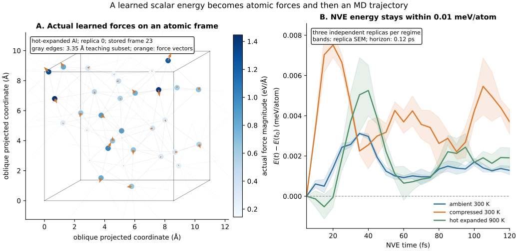
The left panel is not a lattice redrawn from the input CIF. It uses stored frame 23 from the real hot-expanded, replica-0 NVT HDF5 file. Positions are wrapped into the primary cell and shown with an oblique projection so the atomic layers remain visible. The orange vectors come from \(-\texttt{position\_gradients}\), and the color scale reports their full three-dimensional magnitudes in eV/Å.
The gray lines need a careful label. They show pairs within 3.35 Å to make the local graph idea visible. The deployed MACE model has its own serialized cutoff and a richer message-passing graph. The figure does not claim that every gray line—or only those gray lines—was a MACE edge.
The right panel follows what happens after forces enter the integrator. For each NVE replica, total energy per atom is shifted by its first stored value. All three regime means remain within 0.01 meV/atom over 0.12 ps. This is strong short-horizon numerical self-consistency for the selected timestep and visited states. It is not a comparison with density-functional theory.
A stable learned Hamiltonian can still be wrong
For an autonomous NVE system, a conservative force and suitable integrator should produce bounded total-energy error. A line fit to each replica’s total energy per atom gives the following absolute slopes:
| Regime | Absolute NVE drift ± replica SEM (meV/atom/ps) | Energy span ± replica SEM (meV/atom) |
|---|---|---|
| ambient fcc | 0.00126 ± 0.00045 | 0.00321 ± 0.00007 |
| compressed fcc | 0.00446 ± 0.00289 | 0.00819 ± 0.00045 |
| hot expanded fcc | 0.00504 ± 0.00169 | 0.00624 ± 0.00212 |
These numbers test whether the discrete trajectory approximately conserves the Tojax MACE energy that generated it. A smooth but biased learned energy can conserve itself perfectly. Conversely, a good model can show bad drift when the timestep is too large, precision is mishandled, or a neighbor-list update is discontinuous.
The 0.12 ps horizon is part of the result. A slope measured here must not be extrapolated to nanoseconds. Longer paths can enter configurations absent from this test or reveal slow trends that 24 frames cannot show. A timestep scan is also required before calling 0.5 fs converged.
A thermostat setpoint is not a measured temperature
The first production attempt used only 50 fs of NVT warmup with a 100 fs Langevin relaxation scale. Its measured means were about 241, 260, and 693 K for setpoints of 300, 300, and 900 K. Nothing crashed. The trajectories were simply still relaxing.
The accepted protocol warms up for 500 fs—five relaxation times—before its 120 fs measurement window:
| Regime | Setpoint (K) | Measured NVT mean ± replica SEM (K) | Difference (K) |
|---|---|---|---|
| ambient fcc | 300 | 304.4 ± 14.5 | 4.4 |
| compressed fcc | 300 | 304.4 ± 19.0 | 4.4 |
| hot expanded fcc | 900 | 831.9 ± 39.1 | 68.1 |
The two 300 K means are close to their setpoints relative to their three-path spread. The hot mean remains 68 K low, about 1.7 reported SEMs. Replacing that measurement with the 900 K input would turn a request into a result. The appropriate conclusion is that the obvious warmup transient was reduced and the hot regime still needs a longer equilibration and sampling study.
Replica SEM also has a narrow meaning. For a per-replica scalar \(m_r\),
\[\operatorname{SEM}(m) = \frac{s(m_1,m_2,m_3)}{\sqrt{3}}.\]It measures variation among three initialized paths under one model and one protocol. It does not correct time correlation within a path and it does not measure uncertainty in the learned energy.
Force scale and displacement are not force errors
The NVT trajectories also provide potential energy, maximum force, periodic nearest-neighbor distance, and minimum-image RMS displacement:
| Regime | Potential energy ± SEM (eV/atom) | Mean max force ± SEM (eV/Å) | Nearest neighbor ± SEM (Å) | RMS displacement ± SEM (Å) |
|---|---|---|---|---|
| ambient fcc | -3.70402 ± 0.00048 | 1.086 ± 0.052 | 2.6906 ± 0.0002 | 0.1903 ± 0.0004 |
| compressed fcc | -3.37802 ± 0.00194 | 1.703 ± 0.074 | 2.5345 ± 0.0011 | 0.1136 ± 0.0059 |
| hot expanded fcc | -3.51522 ± 0.00306 | 1.856 ± 0.158 | 2.6336 ± 0.0095 | 0.3340 ± 0.0157 |
Within this learned Hamiltonian, compression shortens the measured nearest- neighbor distance and increases the force scale relative to ambient fcc. The hot expanded trajectories have the largest displacement and mean maximum force. These metrics describe the configurations the model generated.
They are not errors because no reference energy or force appears in their definition. Large forces can be a reasonable response to distorted atoms. Small forces can be consistently biased. Reference accuracy requires selected trajectory frames labeled by a higher-level calculation or experiment.
One checkpoint cannot produce epistemic uncertainty
The workflow uses one serialized MACE checkpoint. It has no committee, posterior sample, calibrated representation distance, or residual model. The summary therefore records epistemic_uncertainty_available: false.
The ± values above are replica SEMs. If all three replicas share the same model bias, their SEM can be tiny while the energy surface is wrong. Difficulty is not uncertainty either: a compressed or hot cell may be challenging, but its name is not an extrapolation score.
A defensible support or uncertainty statement could use a calibrated model ensemble, explicit coverage in a relevant local-environment representation, or reference residuals on deployment frames. The calibration target matters. Detecting unusual local geometry, predicting force error, and covering an observable are different tasks.
For this experiment, the next validation set should draw frames from all three regimes. It should be stratified by time, local coordination, and force scale rather than filled with adjacent ambient frames. Reference energies, forces, and stresses would then support actual error metrics and expose whether the distorted regimes fail differently.1
The capstone validation ladder
Every earlier chapter fits into one ordered set of questions:
- Identity and execution: Which artifact, revision, hash, backend, engine, and device produced the force calls?
- Numerical method: Do initialization, units, precision, neighbor updates, and timestep produce stable trajectories?
- Ensemble and sampling: Did warmup finish, are paths independent, and is the effective sample count adequate for the observable?
- Model validity: Are energies, forces, and stresses accurate on the configurations that control the claim?
- Estimator validity: Do histogram support, overlap, bias removal, or work tails support the final observable?
The weakest supported link limits the conclusion. Skipping directly to model RMSE ignores the MD protocol. Stopping after a successful HDF5 write ignores the model and the science.
Enhanced sampling makes this ladder especially important. An umbrella or adaptive bias deliberately visits rare configurations. The estimator can be implemented correctly while reconstructing the free energy of a learned Hamiltonian that has never been validated in the barrier region.
Exercises: decide what each test can prove
For each proposed change, state which rung of the ladder it strengthens:
- Halve the timestep and compare NVE energy spans.
- Run ten replicas of the same checkpoint.
- Evaluate DFT forces on high-force frames from all three regimes.
- Compare two independently trained checkpoints and calibrate their disagreement against the DFT subset.
- Extend the hot NVT run until its temperature mean and autocorrelation-based uncertainty stabilize.
The trap is item 2. More replicas reduce sampling uncertainty under the same learned Hamiltonian. They do not expose a bias shared by that checkpoint. Item 3 tests reference accuracy; item 4 can begin an epistemic-uncertainty study; items 1 and 5 test numerical and sampling claims.
Reproducibility record and full diagnostic dashboard
The public-reviewable artifacts are the smoke configuration, full configuration, notebook, smoke summary, production summary, 432-row sample table, manifest, kUPS/Tojax worker, JAX reference algorithms, atomic-visual source, figure-generation entry point, and review record.
git clone https://github.com/sungsoo-ahn/kups-md-tutorials
cd kups-md-tutorials
uv sync --locked --extra gpu --extra mlff

uv run kups-tutorial run 12 --profile smoke
uv run kups-tutorial verify 12 --profile smoke
uv run kups-tutorial run 12 --profile full
uv run kups-tutorial verify 12 --profile full
uv run python scripts/generate_post12_figures.py
uv run kups-tutorial verify-notebooks --posts 12 --timeout 240
The 18 raw HDF5 files remain outside the website repository. For each one, the manifest preserves regime, replica, ensemble, integrator, seed, requested and observed devices, input CIF hash, raw HDF5 hash and byte count, frame and atom counts, dataset names and dtypes, worker time, and derived metrics. The compact CSV retains every stored frame used above.
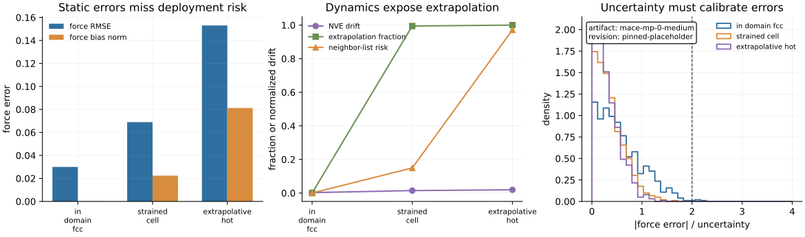
The multi-panel figure below preserves the full temperature, energy-drift, force-scale, and displacement dashboard. It is an audit view, not the main atomic explanation.
What this experiment does not establish
- No DFT or experimental labels were evaluated, so there is no accuracy claim.
- One checkpoint ran, so there is no epistemic-uncertainty claim.
- No support metric was calibrated, so there is no in-domain/extrapolation label.
- The NVE horizon is 0.12 ps, so there is no long-time stability claim.
- The NVT measurement is 0.12 ps with three replicas, so there is no converged material or transport observable.
- NVE starts independently rather than from equilibrated NVT endpoints, so there is no thermostat-to-microcanonical handoff result.
- Only strained fcc Al cells were tested. Defects, surfaces, liquids, multicomponent systems, reactions, and extreme coordination remain outside the evidence.
These boundaries locate the next experiment. A defect barrier needs reference checks along the transition region plus window overlap. A melting claim needs larger cells, longer phase-specific sampling, and validation in both phases. A mechanical-response claim needs stress references and strain-path convergence.
Closing
A learned potential does not enter MD as a picture of a neural network. It enters as a scalar function whose gradients move atoms.
Make that chain visible. Freeze the exported computation. Verify the device and raw trajectory. Test the timestep, ensemble, and sample count. Then obtain reference evidence on the configurations that matter to the final observable. Only after all of those steps should a stable learned trajectory become a physical claim.
References
- Morrow, J. D., Gardner, J. L. A. & Deringer, V. L. (2023). How to validate machine-learned interatomic potentials. The Journal of Chemical Physics, 158, 121501. DOI ↩
- Batatia, I. et al. (2022). MACE: Higher order equivariant message passing neural networks for fast and accurate force fields. arXiv
- Batatia, I. et al. (2025). A foundation model for atomistic materials chemistry. The Journal of Chemical Physics, 163, 184110. DOI
- CuspAI. kUPS documentation.
- CuspAI. Tojax source repository.