A molecular-dynamics trajectory can remain trapped in one free-energy basin for far longer than we can afford to simulate. Enhanced sampling changes the calculation so that rare regions become easier to visit. The dangerous leap is to confuse visiting a region with measuring its equilibrium probability.
This chapter studies two ways of changing the calculation:
- adaptive bias changes the energy landscape according to the trajectory’s accumulated history;
- nonequilibrium steering prescribes a time-dependent protocol and records the work performed along each path.
They solve related sampling problems, but they generate different data and require different estimators. A metadynamics bias history is not a work path. A steered path is not a biased equilibrium histogram. We will implement the central update for each method in JAX, then use real kUPS trajectories to see what a moving restraint actually does to two atoms.
- how a collective variable compresses atomic configurations into a coordinate;
- why well-tempered Gaussian hills become shorter as local bias accumulates;
- why adaptive bias and nonequilibrium steering are distinct sampling procedures;
- how a discrete restraint-center change performs work at a fixed coordinate;
- how kUPS makes the restraint center depend on the MD step;
- why slower pulling can reduce lag and hysteresis without becoming equilibrium;
- how Jarzynski’s equality turns a path ensemble into a tail-sensitive estimate;
- why effective sample size and forward–reverse agreement do not prove convergence.
Prerequisites: biased distributions from Post 08, overlap and exponential weights from Post 09, harmonic restraints from Post 10, and Langevin dynamics from Post 04.
The collapsed setup selects JAX CPU for the teaching kernels and imports the same workflow that launches the real kUPS smoke experiment later.
Python
from pathlib import Path
import os
import warnings

warnings.filterwarnings("ignore", message="IProgress not found")
os.environ.setdefault("JAX_PLATFORMS", "cpu")

import jax
from jax import Array
import jax.numpy as jnp
from IPython.display import Image, display

from kups_md_tutorials.config import load_enhanced_sampling_spec
from kups_md_tutorials.enhanced_sampling import (
    load_enhanced_sampling_summary,
    write_enhanced_sampling_outputs,
)
from kups_md_tutorials.workflows import verify_post

repo_root = Path.cwd()
if not (repo_root / "configs").exists():
    repo_root = repo_root.parent
os.chdir(repo_root)
Part I: adaptive bias remembers where the path has been
Let \(\mathbf R\) collect all atomic positions. A collective variable
\[s=\xi(\mathbf R)\]maps that high-dimensional configuration to a smaller coordinate. It could be an atom-pair distance, a torsion angle, a coordination number, or a learned descriptor. Choosing \(s\) is a scientific assumption: motion hidden from \(s\) can remain slow even when \(s\) appears to move freely.
Metadynamics builds a history-dependent bias by depositing Gaussian hills at previously visited values \(s_i=s(t_i)\):
\[V_t(s) = \sum_{t_i<t} w_i \exp\left[-\frac{(s-s_i)^2}{2\sigma^2}\right].\]Here \(V_t\) is the accumulated bias at time \(t\), \(w_i\) is the height of hill \(i\), and \(\sigma\) is its width in collective-variable units. A new positive hill makes the visited neighborhood less favorable. Repeated hills therefore encourage the path to leave an already explored basin.
The time subscript matters. A fixed umbrella samples one stationary modified Hamiltonian. Metadynamics changes its Hamiltonian while sampling. The path at time \(t\) depends on every earlier deposition event.
Well tempering slows the deposition
Depositing hills of constant height forever would keep forcing the landscape away from a steady limit. Well-tempered metadynamics reduces a new hill using the bias already present at the sampled point:1
\[w_i = w_0 \exp\left[ -\frac{V_{t_i}(s_i)}{k_{\mathrm B}\Delta T} \right], \qquad \gamma=\frac{T+\Delta T}{T}.\]The initial height is \(w_0\), the physical temperature is \(T\), and \(\Delta T=(\gamma-1)T\) sets how quickly hills shrink. Large accumulated bias means a smaller next hill. The dimensionless bias factor \(\gamma\) must exceed one.
The JAX function below performs exactly one deposition event. jnp.interp reads the current local bias, the exponential tempers the height, and the final line adds a Gaussian across the grid.
Python
def well_tempered_gaussian_deposit(
    bias: Array,
    grid: Array,
    sample: Array,
    initial_height: float,
    width: float,
    bias_factor: float,
    thermal_energy: float,
) -> tuple[Array, Array]:
    """Deposit one well-tempered Gaussian hill on a one-dimensional grid."""

    local_bias = jnp.interp(sample, grid, bias)
    tempering_energy = (bias_factor - 1.0) * thermal_energy
    deposited_height = initial_height * jnp.exp(-local_bias / tempering_energy)
    gaussian = jnp.exp(-0.5 * ((grid - sample) / width) ** 2)
    return bias + deposited_height * gaussian, deposited_height


grid = jnp.linspace(-2.5, 2.5, 2001)
empty_bias = jnp.zeros_like(grid)
accumulated_bias = 2.0 * jnp.exp(-0.5 * (grid / 0.12) ** 2)
_, first_height = well_tempered_gaussian_deposit(
    empty_bias, grid, jnp.array(0.0), 0.03, 0.12, 10.0, 1.0
)
_, tempered_height = well_tempered_gaussian_deposit(
    accumulated_bias, grid, jnp.array(0.0), 0.03, 0.12, 10.0, 1.0
)
print(f"first hill at zero bias={float(first_height):.5f}")
print(f"hill after local bias reaches 2 kBT={float(tempered_height):.5f}")first hill at zero bias=0.03000
hill after local bias reaches 2 kBT=0.02402
With no accumulated bias, the deposited height equals the requested 0.03000. When the local bias is already \(2k_{\mathrm B}T\) and \(\gamma=10\), the same request deposits only 0.02402. This is the adaptive mechanism—not yet a free-energy estimate.
In the long-time well-tempered limit, the standard reconstruction is
\[F(s) = -\frac{\gamma}{\gamma-1}V(s)+C,\]where \(C\) is an arbitrary additive constant. The relation is asymptotic. It does not excuse a poor collective variable, an unconverged bias history, or missing support in a hidden slow coordinate.
Test adaptive bias against an answer key
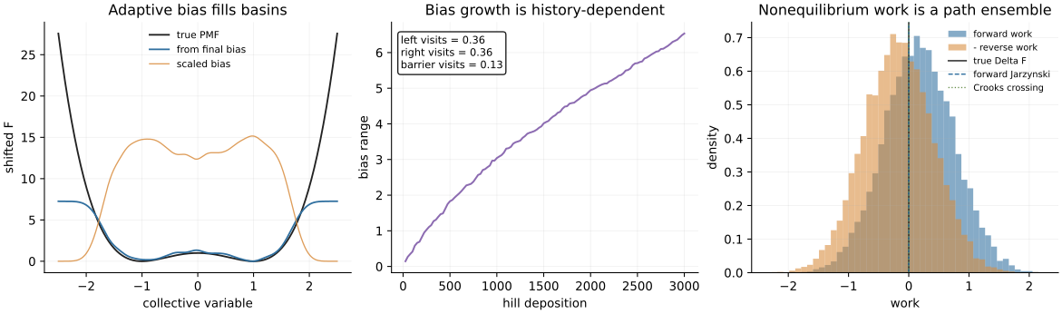
The full analytic control uses a one-dimensional double well whose barrier is known before sampling. It deposits 3,000 hills with \(\gamma=10\). The final bias range is 6.378 reduced-energy units, both basins receive nearly equal support, and the reconstructed barrier differs from the answer by 0.0749.
| Adaptive-bias check | Full value | Interpretation |
|---|---|---|
| deposited hills | 3,000 | length of the history |
| final bias range | 6.378 | the landscape changed substantially |
| left / right basin visits | 0.360 / 0.362 | both basins were explored |
| barrier-region visits | 0.134 | the barrier region gained support |
| barrier-height error | 0.0749 | known-answer reconstruction error |
Equal basin counts alone would not validate the method. The answer-key error does. On a molecular problem without an answer key, repeatability across independent bias histories and stability to hill height, width, bias factor, and deposition interval become essential.
This metadynamics example is an analytic teaching control. The physical kUPS experiment below performs steered MD, not metadynamics. Keeping that boundary explicit prevents evidence from one method being borrowed to support another.
Part II: steering prescribes a protocol
For the kUPS experiment, the collective variable is the minimum-image distance \(r(\mathbf R)\) between two argon atoms. A harmonic restraint has a center \(c(t)\) that moves from 3.8 Å to 7.5 Å:
\[U_{\mathrm{bias}}(\mathbf R,t) = \frac{K}{2}\left[r(\mathbf R)-c(t)\right]^2.\]The restraint center is an energetic preference, not a position constraint. At every MD step, Lennard–Jones forces, thermal noise, inertia, and the bias force jointly determine the next atomic state. The realized distance can lag, overshoot, or fluctuate around the center.
Work occurs when the protocol changes
The implementation keeps the center fixed within each stored MD block. At a block boundary it changes the center from \(c_i\) to \(c_{i+1}\) while holding the stored coordinate \(r_i\) fixed. Work is the instantaneous energy change caused by that parameter update:
\[\Delta W_i = U_{\mathrm{bias}}(r_i,c_{i+1}) -U_{\mathrm{bias}}(r_i,c_i) = \frac{K}{2} \left[ (r_i-c_{i+1})^2-(r_i-c_i)^2 \right].\]The atoms do not move during this accounting event. Coordinate propagation at a fixed center contributes heat and internal-energy change, but not protocol work. The last stored frame has no following center change, so its increment is zero.
Python
def discrete_harmonic_protocol_work(
    distances: Array,
    centers: Array,
    force_constant: float,
) -> Array:
    """Evaluate work from discrete harmonic-center changes at fixed coordinates."""

    old_bias = 0.5 * force_constant * (distances[:-1] - centers[:-1]) ** 2
    new_bias = 0.5 * force_constant * (distances[:-1] - centers[1:]) ** 2
    return jnp.concatenate((new_bias - old_bias, jnp.zeros(1, distances.dtype)))


full_spec = load_enhanced_sampling_spec("11", "full")
steering = full_spec.pair_distance_steered
assert steering is not None
centers = jnp.array([3.8, 5.0, 7.5])
distances = jnp.array([4.0, 4.8, 6.9])
increments = discrete_harmonic_protocol_work(
    distances,
    centers,
    steering.force_constant_ev_per_angstrom2,
)
{
    "stored distance (angstrom)": [round(x, 2) for x in distances.tolist()],
    "restraint center (angstrom)": [round(x, 2) for x in centers.tolist()],
    "protocol-work increment (eV)": [round(x, 6) for x in increments.tolist()],
    "kUPS harmonic k = K/2 (eV/angstrom^2)": (
        0.5 * steering.force_constant_ev_per_angstrom2
    ),
}{'stored distance (angstrom)': [4.0, 4.8, 6.9],
'restraint center (angstrom)': [3.8, 5.0, 7.5],
'protocol-work increment (eV)': [0.0096, 0.0725, 0.0],
'kUPS harmonic k = K/2 (eV/angstrom^2)': 0.01}For the three-event control, the two center changes contribute 0.0096 and 0.0725 eV. The final zero is not padding; it encodes the fact that no later protocol value exists. Summing this array reconstructs the total work from the stored distances and center schedule.
Map that definition to kUPS
The real worker implements the same event sequence:
- read the kUPS MD step counter and select the corresponding center;
- evaluate the harmonic pair restraint with that center;
- add it to the Lennard–Jones energy with
sum_potentials; - obtain forces from the combined energy inside the kUPS propagator;
- advance BAOAB Langevin dynamics with
run_md; - store positions, reconstruct minimum-image distances, and evaluate the JAX work formula above at block boundaries.
kUPS defines its harmonic bond as \(k(r-r_0)^2\), whereas this chapter writes \(K(r-r_0)^2/2\). The worker therefore passes \(k=K/2\). Before production, it compares the dynamic first-center potential with an independently built static restraint in both energy and gradient. It also verifies that zero drive gives zero work and that a kUPS energy difference matches the analytic increment.
Those checks establish the implemented Hamiltonian and accounting convention. They do not show that the protocol is slow or that the path ensemble is large enough.
Run actual steering trajectories
The fresh-kernel notebook launches four CPU-sized kUPS paths: fast and slow protocols in both forward and reverse directions. Each isolated worker constructs the combined potential, propagates real MD, writes HDF5 positions, and returns a compact work trace. The notebook then invokes the same verifier used by the command-line workflow.
Python
smoke_spec = load_enhanced_sampling_spec("11", "smoke")
smoke_dir = write_enhanced_sampling_outputs(
    smoke_spec,
    output_root=Path("notebook-runs"),
    quiet=True,
)
verify_post("11", "smoke", output_root=Path("notebook-runs"))
smoke = load_enhanced_sampling_summary(
    smoke_dir / "enhanced_sampling_summary.json"
)
smoke_pair = smoke.pair_distance_steered
assert smoke_pair is not None
{
    "engine and device": (smoke_pair.engine, smoke_pair.observed_devices),
    "runs / stored frames": (smoke_pair.run_count, smoke_pair.total_frames),
    "fast / slow hysteresis gaps (eV)": (
        round(smoke_pair.fast_hysteresis_gap, 5),
        round(smoke_pair.slow_hysteresis_gap, 5),
    ),
    "zero-drive work error (eV)": smoke_pair.zero_drive_work_error_ev,
    "kUPS work-increment error (eV)": (
        smoke_pair.kups_work_increment_error_ev
    ),
}{'engine and device': ('kups', ('cpu:cpu',)),
'runs / stored frames': (4, 160),
'fast / slow hysteresis gaps (eV)': (0.20316, 0.02302),
'zero-drive work error (eV)': 0.0,
'kUPS work-increment error (eV)': 3.895587141929113e-09}The new smoke run stores 160 frames. Its fast hysteresis gap is 0.2032 eV and its slow gap is 0.0230 eV. Zero drive gives exactly zero work, and the largest kUPS-versus-analytic increment error is \(3.90\times10^{-9}\) eV. This is bounded execution evidence on CPU; the independent-replica GPU record carries the quantitative comparison.
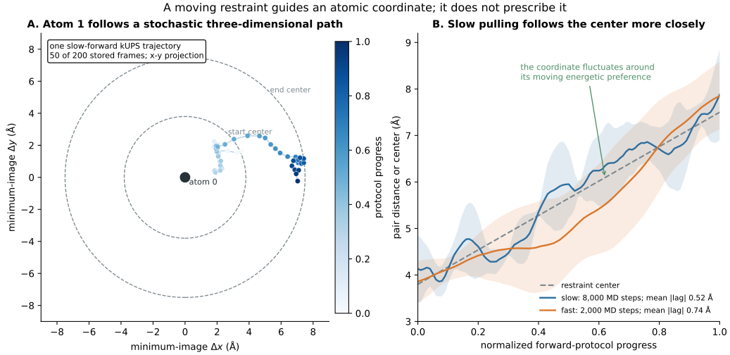
The left panel is an actual atomic trajectory, not a schematic interpolation between the endpoints. The three-dimensional pair displacement is projected onto the x-y plane, so radial pulling and rotational diffusion both appear. The dashed circles show only the initial and final restraint centers.
The right panel separates the protocol from the response. Across the four forward paths, the mean absolute distance-to-center lag is 0.74 Å for fast pulling and 0.52 Å for slow pulling. Slowing the schedule lets the coordinate track its moving preference more closely, but the shaded replica spread makes clear that thermal fluctuations remain.
Hysteresis asks whether slower was actually gentler
For a forward path, the second law implies
\[\langle W_{\mathrm F}\rangle\geq\Delta F.\]For the reverse direction,
\[\langle W_{\mathrm R}\rangle\geq-\Delta F.\]Their sum defines a loop-width diagnostic,
\[H = \langle W_{\mathrm F}\rangle +\langle W_{\mathrm R}\rangle.\]An ideal quasistatic pair of protocols has \(H=0\). Finite-speed driving, coordinate lag, and relaxation hidden from the chosen coordinate make the loop wider. Hysteresis is not itself a free-energy estimator; it answers a more limited question: did allocating more MD steps reduce dissipation?
The full experiment uses two Ar atoms in a periodic 30 Å cube at 100 K, Lennard–Jones parameters \(\sigma=3.405\) Å and \(\epsilon=0.010326\) eV, and \(K=0.02\) eV/Å\(^2\). Four independent replicas are run for every speed–direction combination, giving 16 GPU paths and 2,000 stored frames.
Python
production = load_enhanced_sampling_summary(
    Path("results/post-11/full/enhanced_sampling_summary.json")
)
pair = production.pair_distance_steered
assert pair is not None
{
    "kUPS version / device": (pair.kups_version, pair.observed_devices),
    "replicas / runs / frames": (
        pair.replica_count, pair.run_count, pair.total_frames
    ),
    "fast hysteresis gap +/- SEM (eV)": (
        round(pair.fast_hysteresis_gap, 5),
        round(pair.fast_hysteresis_gap_sem, 5),
    ),
    "slow hysteresis gap +/- SEM (eV)": (
        round(pair.slow_hysteresis_gap, 5),
        round(pair.slow_hysteresis_gap_sem, 5),
    ),
    "fast / slow gap ratio": round(pair.hysteresis_gap_ratio, 2),
    "forward / reverse Jarzynski (eV)": (
        round(pair.forward_jarzynski_delta_f, 5),
        round(pair.reverse_jarzynski_delta_f, 5),
    ),
    "zero-drive / work-increment errors (eV)": (
        pair.zero_drive_work_error_ev, pair.kups_work_increment_error_ev
    ),
}{'kUPS version / device': ('1.0.3', ('gpu:NVIDIA RTX A5000',)),
'replicas / runs / frames': (4, 16, 2000),
'fast hysteresis gap +/- SEM (eV)': (0.05258, 0.026),
'slow hysteresis gap +/- SEM (eV)': (0.01113, 0.00866),
'fast / slow gap ratio': 4.72,
'forward / reverse Jarzynski (eV)': (-0.01126, -0.01238),
'zero-drive / work-increment errors (eV)': (0.0, 6.815571232388073e-10)}| Production check | Full-profile value | What it supports |
|---|---|---|
| observed device | NVIDIA RTX A5000 | required GPU execution |
| fast hysteresis | 0.05258 ± 0.02600 eV | four-path mean and path SEM |
| slow hysteresis | 0.01113 ± 0.00866 eV | smaller than fast |
| fast / slow ratio | 4.72 | slower protocol narrows this loop |
| static energy / gradient error | 0 / 0 | dynamic first center matches static bias |
| zero-drive work error | 0 eV | no parameter change means no work |
| maximum work-increment error | \(6.82\times10^{-10}\) eV | stored-frame accounting matches kUPS |
The uncertainty is not decorative. One fast-forward replica records 0.0848 eV of work while another records -0.0205 eV. Four paths support the limited claim that this slower protocol reduces the loop width in this teaching system. They do not determine the tails of a work distribution precisely.
Jarzynski is exact and tail-sensitive
Jarzynski’s equality relates a nonequilibrium path ensemble to the equilibrium free-energy difference:2
\[e^{-\beta\Delta F} = \left\langle e^{-\beta W}\right\rangle, \qquad \beta=\frac{1}{k_{\mathrm B}T}.\]The average is over independently initialized paths generated by the same protocol. Taking the logarithm gives the finite-sample estimator
\[\widehat{\Delta F} = -k_{\mathrm B}T \log\left[ \frac{1}{N}\sum_{n=1}^{N} e^{-W_n/(k_{\mathrm B}T)} \right].\]Low-work paths receive exponentially larger weights. Numerically, the JAX implementation uses logsumexp so tiny weights do not underflow. It also reports the normalized effective sample size
Python
def jarzynski_free_energy_and_ess(
    work: Array,
    thermal_energy: float,
) -> tuple[Array, Array]:
    """Estimate a physical free-energy difference and exponential-weight ESS."""

    log_weights = -work / thermal_energy
    log_mean_weight = jax.scipy.special.logsumexp(log_weights) - jnp.log(work.size)
    delta_free_energy = -thermal_energy * log_mean_weight
    shifted_weights = jnp.exp(log_weights - jnp.max(log_weights))
    effective_samples = jnp.sum(shifted_weights) ** 2 / jnp.sum(shifted_weights**2)
    return delta_free_energy, effective_samples / work.size


constant_work = jnp.full(12, 0.07)
delta_f, ess_fraction = jarzynski_free_energy_and_ess(
    constant_work, thermal_energy=0.025
)
print(f"known work / estimated delta F={float(constant_work[0]):.3f} / {float(delta_f):.3f} eV")
print(f"exponential-weight ESS={float(ess_fraction):.3f} of the 12 paths")known work / estimated delta F=0.070 / 0.070 eV
exponential-weight ESS=1.000 of the 12 paths
When all 12 control paths have the same work, Jarzynski must return that work and every path carries equal weight. The output recovers 0.070 eV and an ESS fraction of 1.000. Real nonequilibrium work is neither constant nor so kind.
For the radial Ar-pair answer key, \(\Delta F=-0.00570\) eV between the two restrained endpoints. Only four slow paths per direction give forward and reverse Jarzynski estimates of -0.01126 and -0.01238 eV. They agree with each other to 0.00112 eV, yet both miss the answer by roughly 0.006–0.007 eV. The ESS fractions are 0.546 and 0.672.
This is the central warning: directional agreement and a moderate ESS do not manufacture an unsampled exponential tail. A defensible free-energy claim would need more independent equilibrated starting states, path-count and tail stability tests, and preferably a bidirectional estimator using forward–reverse overlap.3
A prediction to test
Before changing code, predict the effect of each intervention:
- Halve the metadynamics hill width while keeping its height fixed. Which parts of the reconstructed free energy should become noisier?
- Double the number of MD steps in the slow steering protocol without changing its endpoints. Should the restraint-center lag, hysteresis, and thermal trajectory spread all decrease in the same way?
- Add many typical-work paths but no unusually low-work paths. Can the ordinary work mean stabilize while the Jarzynski estimate remains biased?
The useful answer to the second question is “not necessarily.” Slower driving should reduce systematic lag and dissipation, but it does not remove equilibrium thermal fluctuations. For the third, Jarzynski can remain unstable because its information lives in a different tail than the ordinary mean.
Reproducibility record and full diagnostic dashboard
The committed source of truth includes the smoke configuration, full configuration, notebook, smoke summary, production summary, stored steering trace, manifest, kUPS worker, JAX reference algorithms, figure source, figure-generation entry point, and review record.
uv run kups-tutorial run 11 --profile smoke
uv run kups-tutorial verify 11 --profile smoke
uv run kups-tutorial run 11 --profile full
uv run kups-tutorial verify 11 --profile full
uv run kups-tutorial verify-notebooks --posts 11 --timeout 180
Each of the 16 production paths records the input CIF and HDF5 SHA-256, raw byte count and dataset schema, seed, speed, direction, replica, frame count, observed device, runtime, block thermodynamics, and work controls. The compact CSV retains every center, distance, work increment, and cumulative work value. The figure provenance records the selected HDF5 hash, frame indices, minimum-image convention, projection, and all-forward-replica trace hash.
The multi-panel dashboard below preserves the analytic work controls, complete metadynamics reconstruction, driven-coordinate traces, and cumulative work. It is useful for audit, but the two-panel atomic figure carries the main physical argument.
What this chapter establishes—and what it does not
The adaptive control shows that the standard well-tempered update can fill and approximately reconstruct a known double well. It does not show that kUPS ran metadynamics on an atomistic system.
The physical experiment shows that kUPS ran a time-dependent harmonic restraint on real Ar-pair trajectories, that work is reconstructible at the actual discrete parameter changes, and that a slower schedule reduced lag and forward–reverse hysteresis. It does not show that four paths converge an exponential-work free energy or that pair distance is a challenging reaction coordinate.
That separation is the point. Enhanced sampling is trustworthy when the modified dynamics, stored evidence, and estimator correspond to the same mathematical experiment.
Closing
Adaptive bias and steering both make rare motion easier by changing the measure that generates trajectories. The correction must match the change.
For metadynamics, preserve and test the bias history. For steered MD, define work at the same protocol events the code executes and collect an ensemble of independent paths. In both cases, a visually successful crossing is only the beginning. The result starts when you can explain what distribution generated the data and why the estimator has support there.
References
- Barducci, A., Bussi, G. & Parrinello, M. (2008). Well-tempered metadynamics: A smoothly converging and tunable free-energy method. Physical Review Letters 100, 020603. ↩
- Jarzynski, C. (1997). Nonequilibrium equality for free energy differences. Physical Review Letters 78, 2690. ↩
- Crooks, G. E. (1999). Entropy production fluctuation theorem and the nonequilibrium work relation for free energy differences. Physical Review E 60, 2721. ↩