An ordinary trajectory spends most of its time in low-free-energy basins. If a distance, angle, or other collective variable rarely crosses the region we care about, waiting longer may be an expensive way to collect almost no new information there.
Umbrella sampling changes the Hamiltonian on purpose. Several simulations add different harmonic biases, so each one visits a local range of the collective variable. A reconstruction such as WHAM then removes the known biases and aligns the windows through their shared probability.
The word shared is the entire method. A smooth reconstructed PMF can still be unsupported if one adjacent pair of windows does not overlap. We will make the complete chain visible: a minimum-image atom-pair distance, its harmonic bias, forces from jax.grad, the equivalent kUPS potential composition, real biased trajectories, and the WHAM fixed-point equations that combine their histograms.
- why an umbrella window samples a biased ensemble rather than a target value;
- how a pair-distance bias acts on two atomic positions under periodic boundaries;
- how JAX differentiates the bias into equal-and-opposite atomic forces;
- how kUPS composes the restraint with the physical potential and propagates MD;
- how WHAM solves for one unbiased density and one offset per window;
- why adjacent overlap, replica agreement, and coordinate measure are separate checks;
- how an apparently successful sparse reconstruction fails a known-answer test.
Prerequisites: biased reweighting from Post 08, estimator overlap from Post 09, periodic distances from Post 07, and Langevin sampling from Post 04.
A window samples a modified Hamiltonian
Let \(s(\mathbf R)\) be a collective variable computed from all atomic positions \(\mathbf R\). Window \(i\) adds a harmonic bias centered at \(s_i\),
\[V_i(s)=\frac{K}{2}(s-s_i)^2,\]where \(K\) is the force constant. If the unbiased free energy along the coordinate is \(F(s)\), the window samples
\[p_i(s)\propto \exp\left\{-\beta\left[F(s)+V_i(s)\right]\right\}, \qquad \beta=\frac{1}{k_{\mathrm B}T}.\]The center \(s_i\) is not a command that the coordinate equal \(s_i\). It is the minimum of the added bias. The slope of the underlying free energy, thermal fluctuations, boundaries, and hidden slow coordinates all move or distort the sampled distribution. Window centers describe the protocol; the resulting histograms describe the evidence.
The bias also changes the ensemble. A histogram from one window is not the unbiased probability. Because \(V_i\) is known, its effect can be removed—but only where that window actually generated samples.
Put the harmonic restraint on atoms
This tutorial biases the minimum-image distance between two argon atoms. For a cubic box of length \(L\), first wrap their displacement component by component,
\[\mathbf d =\mathbf R_1-\mathbf R_0 -L\,\operatorname{round}\!\left(\frac{\mathbf R_1-\mathbf R_0}{L}\right), \qquad r=\lVert\mathbf d\rVert.\]The umbrella energy is \(V_i(r)=K(r-r_i)^2/2\). Away from \(r=0\), its forces are
\[\mathbf F_1^{\mathrm{bias}} =-K(r-r_i)\frac{\mathbf d}{r}, \qquad \mathbf F_0^{\mathrm{bias}}=-\mathbf F_1^{\mathrm{bias}}.\]If the atoms are farther apart than the center, the bias pulls them together. If they are closer, it pushes them apart. The net internal bias force is zero, so this restraint does not accelerate the pair’s center of mass.
The collapsed setup selects JAX CPU and imports the real kUPS workflow used later.
Python
from pathlib import Path
import os
import warnings

warnings.filterwarnings("ignore", message="IProgress not found")
os.environ.setdefault("JAX_PLATFORMS", "cpu")

import jax
from jax import Array
import jax.numpy as jnp
from IPython.display import Image, display

from kups_md_tutorials.config import load_umbrella_spec
from kups_md_tutorials.umbrella_sampling import (
    load_umbrella_summary,
    write_umbrella_outputs,
)
from kups_md_tutorials.workflows import verify_post

repo_root = Path.cwd()
if not (repo_root / "configs").exists():
    repo_root = repo_root.parent
os.chdir(repo_root)
The next cell implements the energy exactly as written above. jax.grad differentiates with respect to both atomic positions; no hand-coded force is used by the teaching control.
Python
def periodic_pair_umbrella_energy(
    positions: Array,
    box_lengths: Array,
    center: float,
    force_constant: float,
) -> Array:
    """Evaluate a harmonic pair-distance bias with the minimum-image rule."""

    displacement = positions[1] - positions[0]
    displacement -= box_lengths * jnp.round(displacement / box_lengths)
    distance = jnp.linalg.norm(displacement)
    return 0.5 * force_constant * (distance - center) ** 2


positions = jnp.array([[1.0, 1.0, 1.0], [4.6, 1.0, 1.0]])
box_lengths = jnp.array([30.0, 30.0, 30.0])
bias_energy = periodic_pair_umbrella_energy(positions, box_lengths, 3.4, 0.015)
bias_forces = -jax.grad(periodic_pair_umbrella_energy)(
    positions, box_lengths, 3.4, 0.015
)
print(f"bias energy={float(bias_energy):.6f} eV")
print(f"force on atom 1={bias_forces[1].tolist()} eV/angstrom")
print(f"net bias force={jnp.sum(bias_forces, axis=0).tolist()} eV/angstrom")bias energy=0.000300 eV
force on atom 1=[-0.0029999969992786646, -0.0, -0.0] eV/angstrom
net bias force=[0.0, 0.0, 0.0] eV/angstrom
The atoms are 3.6 Å apart, 0.2 Å beyond a 3.4 Å center, with \(K=0.015\) eV/Å\(^2\). The reported bias is therefore \(K(0.2)^2/2=0.000300\) eV. Atom 1 feels \(-0.0030\) eV/Å along the pair axis, atom 0 feels the opposite force, and their sum is exactly zero in the output.
Match the kUPS energy convention
The production calculation uses the same physics through kUPS. The worker:
- builds the Lennard–Jones base potential with
LjPotentialConfig; - builds a fixed-edge harmonic bond between particle IDs 0 and 1;
- combines them with
sum_potentials; - passes the combined potential to
make_md_propagatorwithbaoab_langevin; - runs warmup and production through
run_mdand stores HDF5 trajectories.
There is one convention worth testing explicitly. The tutorial equation uses \(K(r-r_i)^2/2\), while the kUPS harmonic bond uses \(k(r-r_i)^2\). The worker therefore passes
\[k=\frac{K}{2}.\]A factor-of-two error would still produce smooth trajectories and a smooth PMF. The workflow guards against that kind of silent implementation mistake in two ways. At zero restraint strength, composing the bias must change neither the base energy nor its position gradient. At nonzero strength, the analytic kUPS gradient must agree with a central finite difference. These controls test the Hamiltonian that was implemented; overlap and replicas later test the sampling it produced.
WHAM aligns histograms through shared support
Divide the coordinate into bins \(b\) of width \(\Delta s\). Let \(n_{ib}\) be the count from window \(i\) in bin \(b\), \(N_i=\sum_b n_{ib}\), and \(V_{ib}=V_i(s_b)\). WHAM solves two coupled equations:
\[P_b = \frac{\sum_i n_{ib}} {\sum_i N_i\exp\left[\beta(f_i-V_{ib})\right]},\]and
\[e^{-\beta f_i} =\sum_b P_b e^{-\beta V_{ib}}\Delta s.\]Here \(P_b\) is the reconstructed unbiased probability density and \(f_i\) is the free-energy offset that normalizes window \(i\) relative to the global density. Adding the same constant to all offsets changes nothing, so the code sets the first offset to zero after every update.
These are the standard weighted-histogram self-consistency equations (Kumar et al., 1992).
These equations form a fixed point. Start with offsets, compute \(P_b\), update the offsets from \(P_b\), and repeat. The implementation below performs the calculation in log space. logsumexp prevents overflow in the denominator and normalizations. Bins with zero total counts remain unsupported rather than becoming an arbitrary high PMF.
Python
def wham_fixed_point_pmf(
    counts: Array,
    bias_energies: Array,
    bin_width: float,
    thermal_energy: float,
    *,
    iterations: int = 2000,
) -> tuple[Array, Array, Array]:
    """Reconstruct a supported PMF with log-space WHAM fixed-point updates."""

    sample_counts = jnp.sum(counts, axis=1)
    total_counts = jnp.sum(counts, axis=0)
    log_sample_counts = jnp.log(sample_counts)
    log_total_counts = jnp.where(total_counts > 0.0, jnp.log(total_counts), -jnp.inf)
    log_bin_width = jnp.log(bin_width)

    def update_offsets(_: int, offsets: Array) -> Array:
        log_denominator = jax.scipy.special.logsumexp(
            log_sample_counts[:, None]
            + offsets[:, None] / thermal_energy
            - bias_energies / thermal_energy,
            axis=0,
        )
        log_density = log_total_counts - log_denominator
        log_density -= jax.scipy.special.logsumexp(log_density + log_bin_width)
        log_biased_norms = jax.scipy.special.logsumexp(
            log_density[None, :]
            - bias_energies / thermal_energy
            + log_bin_width,
            axis=1,
        )
        new_offsets = -thermal_energy * log_biased_norms
        return new_offsets - new_offsets[0]

    offsets = jax.lax.fori_loop(
        0,
        iterations,
        update_offsets,
        jnp.zeros(counts.shape[0]),
    )
    log_denominator = jax.scipy.special.logsumexp(
        log_sample_counts[:, None]
        + offsets[:, None] / thermal_energy
        - bias_energies / thermal_energy,
        axis=0,
    )
    log_density = log_total_counts - log_denominator
    log_density -= jax.scipy.special.logsumexp(log_density + log_bin_width)
    supported = total_counts > 0.0
    raw_pmf = -thermal_energy * log_density
    reference = jnp.min(jnp.where(supported, raw_pmf, jnp.inf))
    pmf = jnp.where(supported, raw_pmf - reference, jnp.nan)
    return pmf, supported, offsets


grid = jnp.linspace(-2.0, 2.0, 81)
target_pmf = (grid**2 - 1.0) ** 2
window_centers = jnp.linspace(-1.6, 1.6, 9)
biases = 0.5 * 12.0 * (grid[None, :] - window_centers[:, None]) ** 2
exact_counts = 100_000.0 * jax.nn.softmax(-(target_pmf[None, :] + biases), axis=1)
reconstructed, supported, offsets = wham_fixed_point_pmf(
    exact_counts, biases, float(grid[1] - grid[0]), thermal_energy=1.0
)
error = reconstructed - (target_pmf - jnp.min(target_pmf))
print(f"windows x bins={exact_counts.shape}, supported={int(jnp.sum(supported))}/81")
print(f"known-answer maximum error={float(jnp.nanmax(jnp.abs(error))):.2e}")
print(f"window free-offset range={float(jnp.ptp(offsets)):.3f}")windows x bins=(9, 81), supported=81/81
known-answer maximum error=2.86e-06
window free-offset range=1.182
The exact-count control uses nine harmonic windows over the known double well \(F(s)=(s^2-1)^2\). All 81 bins are supported, and the reconstructed PMF agrees with the answer to \(2.86\times10^{-6}\) in reduced units. This near-exact result validates the equations and their JAX translation. It does not validate a finite trajectory, whose histogram counts are noisy and may be disconnected.
Production WHAM implementations may add convergence tolerances, statistical inefficiency corrections, unequal sample handling, uncertainty estimates, and more robust solvers. The fixed-iteration teaching function exposes the central calculation without claiming to replace those features.
Run actual biased trajectories with kUPS
The smoke profile is a bounded execution test. It launches eight isolated CPU kUPS workers, composes the real base and harmonic potentials, integrates BAOAB Langevin dynamics, reads minimum-image distances from the new HDF5 files, runs the tutorial WHAM analysis, and invokes the same verifier used by the command line.
Python
smoke_spec = load_umbrella_spec("10", "smoke")
smoke_dir = write_umbrella_outputs(
    smoke_spec,
    output_root=Path("notebook-runs"),
)
verify_post("10", "smoke", output_root=Path("notebook-runs"))
smoke = load_umbrella_summary(smoke_dir / "umbrella_summary.json")
smoke_pair = smoke.pair_distance_umbrella
assert smoke_pair is not None
{
    "engine and device": (smoke_pair.engine, smoke_pair.observed_devices),
    "stored frames": smoke_pair.total_frames,
    "minimum adjacent overlap": round(smoke_pair.min_adjacent_overlap, 3),
    "radial-PMF RMSE (eV)": round(smoke_pair.pmf_rmse_vs_true, 5),
    "zero-bias energy error (eV)": smoke_pair.zero_bias_energy_error_ev,
    "force finite-difference error (eV/angstrom)": (
        smoke_pair.bias_force_finite_difference_max_error_ev_per_angstrom
    ),
}{'engine and device': ('kups', ('cpu:cpu',)),
'stored frames': 2400,
'minimum adjacent overlap': 0.143,
'radial-PMF RMSE (eV)': 0.01075,
'zero-bias energy error (eV)': 0.0,
'force finite-difference error (eV/angstrom)': 1.6696285456418991e-06}The fresh run records 2,400 frames. Its minimum adjacent overlap is 0.143 and its radial-PMF RMSE is 0.01075 eV. Those values are useful execution diagnostics, not the physical result: the short CPU profile has one replica and a deliberately small sampling budget. It proves that the current kUPS path runs; the full profile below carries the scientific gates.
Sparse windows can fail with many samples
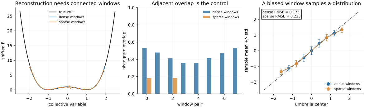
Before interpreting argon, the workflow tests window placement on the same known double well used above. Dense and sparse protocols share the target PMF, temperature, restraint strength, and 20,000 samples per window. Only their centers differ.
| Protocol | Windows | Minimum adjacent overlap | Barrier error | PMF RMSE | Replica PMF RMSE |
|---|---|---|---|---|---|
| dense | 9 | 0.3552 | 0.0106 | 0.1730 | 0.1148 |
| sparse | 4 | 0.0003 | -0.2554 | 0.2229 | 0.2352 |
The sparse grid jumps directly from \(-0.8\) to \(0.8\) across the barrier. Its weakest adjacent overlap is essentially zero. WHAM still returns a finite, smooth curve, but its barrier is too low by 0.255. The code did not crash because disconnected offsets are an identifiability failure, not necessarily a numerical failure.
WHAM and its multistate relative MBAR can combine connected states efficiently; neither supplies probability across an unsampled edge (Shirts & Chodera, 2008).
The global PMF RMSE makes this look milder than it is: sparse RMSE is about 29% worse, while the barrier error is about 24 times larger. A local overlap diagnostic identifies both the cause and the location of the failure.
Watch the atom pair move through connected shells
The physical system is deliberately minimal: two Ar atoms in a periodic 30 Å cube at 100 K, with Lennard–Jones parameters \(\sigma=3.405\) Å and \(\epsilon=0.010326\) eV. Eight umbrella centers span 3.40–7.95 Å with \(K=0.015\) eV/Å\(^2\).
The left panel below uses 100 stored frames from full replica 0 at centers 3.40, 5.35, and 7.95 Å. Atom 0 is placed at the origin and atom 1 is shown at its actual minimum-image displacement, projected from three dimensions into the page. Dashed circles mark the requested bias centers. The arcs rather than perfect circles are real finite-trajectory orientation sampling, not schematic decoration.
The right panel uses all 12,800 pair distances from all eight windows and both replicas. Each ridge is normalized only for visual height; overlap values are computed from the recorded normalized histograms. The weakest edge still has 0.455 shared probability, so the chain remains connected.
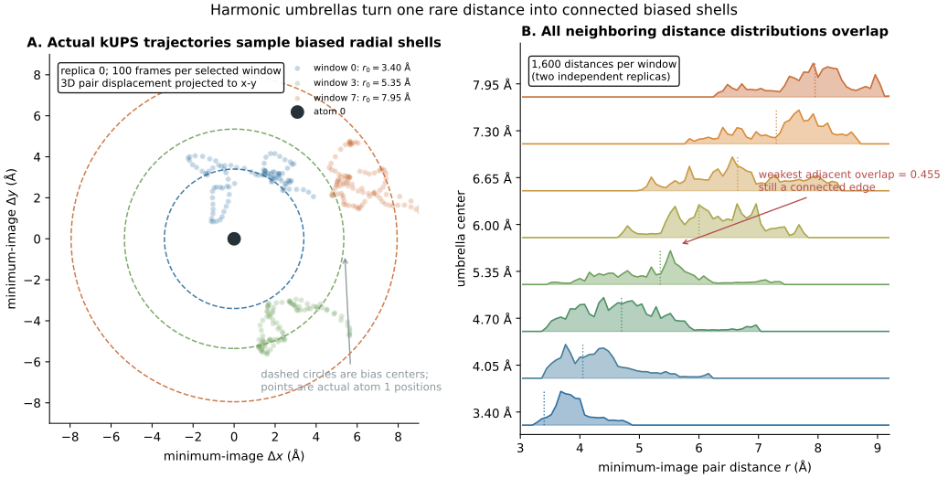
The selected atom clouds explain what the restraint does. They are not the WHAM input by themselves. The reconstruction uses every recorded distance from both replicas and every window.
A radial coordinate carries a geometric measure
For two particles in three dimensions, the number of displacement vectors with length between \(r\) and \(r+dr\) grows as the spherical shell area \(4\pi r^2\). Even if the bare interaction is \(U_{\mathrm{LJ}}(r)\), the scalar distance probability satisfies
\[p(r)\propto r^2e^{-\beta U_{\mathrm{LJ}}(r)}.\]The corresponding radial PMF is
\[F_r(r)=U_{\mathrm{LJ}}(r)-2k_{\mathrm B}T\log r+C.\]WHAM reconstructs this radial PMF because its histograms count scalar pair distances. It should therefore be compared with the radial answer key, not directly with the bare Lennard–Jones interaction. To assess the interaction well, the workflow adds \(2k_{\mathrm B}T\log r\) back, shifts the result, and then measures the recovered well depth.
This distinction is the same Jacobian issue encountered in Post 08: probability in a coordinate and correlation relative to its geometric measure are not the same free-energy convention.
Require overlap and independent replicas
Each full-profile window has two independently seeded trajectories. Every run uses 3,000 warmup steps followed by 8,000 production steps at 1 fs and stores every tenth step, giving 800 frames per run. The complete record contains 8 windows × 2 replicas × 800 frames = 12,800 frames. Every worker observed the required GPU device.
Python
production = load_umbrella_summary(
    Path("results/post-10/full/umbrella_summary.json")
)
pair = production.pair_distance_umbrella
assert pair is not None
{
    "kUPS version": pair.kups_version,
    "observed device": pair.observed_devices,
    "windows x replicas x frames/run": (
        pair.window_count, pair.replica_count, pair.frames_per_run
    ),
    "minimum adjacent overlap": round(pair.min_adjacent_overlap, 4),
    "independent-replica PMF RMSE (eV)": round(
        pair.forward_reverse_pmf_rmse, 5
    ),
    "radial-PMF RMSE (eV)": round(pair.pmf_rmse_vs_true, 5),
    "LJ well-depth error (eV)": round(pair.well_depth_error, 5),
    "zero-bias energy / gradient errors": (
        pair.zero_bias_energy_error_ev,
        pair.zero_bias_gradient_max_error_ev_per_angstrom,
    ),
    "force finite-difference error (eV/angstrom)": (
        pair.bias_force_finite_difference_max_error_ev_per_angstrom
    ),
}{'kUPS version': '1.0.3',
'observed device': ('gpu:NVIDIA RTX A5000',),
'windows x replicas x frames/run': (8, 2, 800),
'minimum adjacent overlap': 0.455,
'independent-replica PMF RMSE (eV)': 0.00407,
'radial-PMF RMSE (eV)': 0.00359,
'LJ well-depth error (eV)': 0.00296,
'zero-bias energy / gradient errors': (0.0, 0.0),
'force finite-difference error (eV/angstrom)': 2.38930806517601e-06}The full evidence passes all declared gates:
| Check | Full-profile value | Gate |
|---|---|---|
| observed device | NVIDIA RTX A5000 | GPU required |
| minimum adjacent overlap | 0.4550 | > 0.20 |
| radial-PMF RMSE | 0.00359 eV | ≤ 0.01 eV |
| independent-replica PMF RMSE | 0.00407 eV | ≤ 0.01 eV |
| corrected LJ well-depth error | 0.00296 eV | ≤ 0.005 eV |
| largest window replica-mean shift | 0.326 Å | ≤ 0.50 Å |
| zero-bias energy / gradient error | 0 / 0 | near zero |
| bias force finite-difference error | \(2.39\times10^{-6}\) eV/Å | ≤ \(10^{-4}\) eV/Å |
The reconstructed radial PMF minimum is at 3.85 Å. Its RMSE against the analytic two-particle radial answer is 3.59 meV, and reconstructing the two replica groups separately changes the PMF by 4.07 meV RMS. After removing the radial measure, the Lennard–Jones well-depth error is 2.96 meV.
These are controlled two-atom results, not a claim that 12,800 frames would converge a complex molecular reaction coordinate. In a larger system, slow orthogonal coordinates can remain trapped even when the one-dimensional umbrella histograms overlap.
Failed pilots are part of the protocol design
The final centers and friction were not assumed to work. An early smoke grid contained a zero-overlap edge. A later GPU protocol met loose scalar PMF gates but showed an approximately 1 Å difference between replica means in one soft window. That disagreement revealed incomplete coordinate relaxation.
Reducing the Langevin friction from 0.01 to 0.002 fs\(^{-1}\) and rerunning both profiles produced the accepted evidence: minimum overlap increased to 0.455 and independent-replica PMF disagreement fell to 0.00407 eV.
This does not mean “lower friction is always better.” It means the diagnostic identified a specific relaxation problem, the protocol changed, and every affected run was regenerated. Failed pilots should change the sampling design, not disappear behind the final curve.
Respond to the diagnostic that actually failed
| Symptom | Likely issue | Useful response |
|---|---|---|
| adjacent overlap near zero | windows too far apart or too stiff | add or move windows; consider broader restraints |
| mean far from its center | strong PMF slope or a boundary | inspect the full distribution before moving the center |
| replica means disagree | slow relaxation or hidden states | extend or redesign equilibration; inspect orthogonal coordinates |
| local histograms look stable but PMFs disagree | offsets are weakly identified | improve the overlap network rather than averaging the conflict |
| statistical checks pass but forces are wrong | bias composition bug | stop and fix zero-bias and finite-difference controls |
| biased structures leave the MLIP domain | model extrapolation | evaluate model validity on those structures or narrow the claim |
Longer sampling helps when overlapping tails exist but are noisy. It does not repair a geometric gap between ensembles. A weaker spring broadens a window, but it may also reduce local control and expose a hidden slow mode. Centers, force constants, initialization, warmup, friction, and production length are one coupled design.
This emphasis on coordinate choice, window design, reconstruction, and convergence evidence is also central to practical umbrella-sampling reviews (Kästner, 2011).
Check your understanding
- If a pair lies 0.2 Å beyond its umbrella center, what happens to the two atomic bias forces?
- Why is a window’s sample mean generally different from its bias center?
- In the WHAM equations, what physical role do the offsets \(f_i\) play?
- Why can WHAM return a smooth curve across a nearly zero-overlap edge?
- Why must a distance PMF include a radial-measure correction before it is compared with a bare pair potential?
The first answer is that the two forces have equal magnitude, point toward restoring the target distance, and sum to zero. The others distinguish biased equilibrium, window normalization, identifiability, and coordinate geometry.
An umbrella is a sampling rule, not evidence of coverage
Umbrella sampling replaces one rare transition with several biased local sampling problems. JAX makes the two core operations explicit: differentiate the bias on atomic coordinates, then solve the WHAM normalization equations. kUPS supplies the actual biased trajectories to which those equations apply.
Trust the reconstructed PMF only when the implemented bias preserves the base Hamiltonian it claims to augment, neighboring windows form a connected overlap network, independent replicas agree, the coordinate measure is handled correctly, and the sampled configurations remain physically and model-theoretically credible.
Reproducibility record and complete umbrella dashboard
Run and verify the bounded CPU profile from the locked environment:
git clone https://github.com/sungsoo-ahn/kups-md-tutorials
cd kups-md-tutorials
uv sync --locked

uv run kups-tutorial run 10 --profile smoke
uv run kups-tutorial verify 10 --profile smoke
uv run kups-tutorial verify-notebooks --posts 10 --output-dir notebook-runs
uv run kups-tutorial export-notebook-cells \
  --executed-notebooks-dir notebook-runs \
  --site-root ../sungsoo-ahn.github.io --posts 10 --check
The full profile requires a working JAX GPU runtime and launches 16 kUPS trajectories:
uv run kups-tutorial run 10 --profile full
uv run kups-tutorial verify 10 --profile full
uv run python scripts/generate_post10_figures.py
Raw HDF5 files remain outside the site repository, but each run record retains its input hash, HDF5 hash and byte count, dataset names/shapes/dtypes, seed, center, frame count, devices, elapsed time, block thermodynamics, and force controls. The compact distance table retains every sample used by WHAM, and the manifest hashes it together with the summary, curves, and window table.
The complete diagnostic dashboard keeps the dense/sparse double-well controls, barrier error, replica disagreement, physical radial PMF, analytic answer, and runtime/force evidence:
Source and evidence:
References
- Kumar, S., Rosenberg, J. M., Bouzida, D., Swendsen, R. H. & Kollman, P. A. (1992). The weighted histogram analysis method for free-energy calculations on biomolecules. Journal of Computational Chemistry, 13, 1011–1021. ↩
- Shirts, M. R. & Chodera, J. D. (2008). Statistically optimal analysis of samples from multiple equilibrium states. The Journal of Chemical Physics, 129, 124105. ↩
- Kästner, J. (2011). Umbrella sampling. WIREs Computational Molecular Science, 1, 932–942. ↩