A free-energy estimator is a way to compare two probability distributions using configurations sampled from one or both of them. Its answer may look precise even when the configurations carrying nearly all of the statistical weight appeared only a handful of times.
That is the trap in this chapter. We will hold the exact free-energy difference fixed while pulling two distributions apart. The nominal sample count remains 50,000, but the useful weighted count falls from 38,949 to 137. A short JAX implementation will expose the exponential weights used by free-energy perturbation (FEP), measure their concentration, and solve the bidirectional Bennett acceptance-ratio (BAR) equation.
The controls are deliberately one-dimensional, so the estimator can be tested against a known answer. They are not molecular trajectories. We will then identify exactly where kUPS enters a molecular calculation and verify the hash-pinned GPU trajectories reused from Post 08.
- what a free-energy difference compares;
- how FEP follows from a ratio of partition functions;
- why exponential averaging is controlled by rare configurations;
- how to implement stable FEP, weight ESS, and equal-sample BAR in JAX;
- why using both directions improves efficiency but cannot replace overlap;
- how MD sampling, cross-state energy evaluation, and estimation fit together;
- why a chain of intermediate states fails when even one link is disconnected.
Prerequisites: relative free energy and reweighting from Post 08, effective sample size from Post 06, and canonical sampling from Post 04.
Two states mean two probability distributions
State A and state B might differ in a force-field parameter, an alchemical coupling, a restrained coordinate, or a molecular identity. At the same temperature, define their reduced potentials
\[u_A(mathbf R)=\beta U_A(mathbf R), \qquad u_B(mathbf R)=\beta U_B(mathbf R), \qquad \beta=\frac{1}{k_{\mathrm B}T}.\]Here \(\mathbf R\) contains all atomic positions and \(U\) has energy units. Multiplication by \(\beta\) makes \(u\) dimensionless. Each state assigns a Boltzmann probability to the same configuration space,
\[p_A(\mathbf R)=\frac{e^{-u_A(\mathbf R)}}{Z_A}, \qquad Z_A=\int d\mathbf R\,e^{-u_A(\mathbf R)},\]and similarly for B. The target is the reduced free-energy difference
\[\Delta f=f_B-f_A=-\log\frac{Z_B}{Z_A}.\]The physical free-energy difference is \(\Delta F=k_{\mathrm B}T\Delta f\). This chapter reports reduced, dimensionless values because its controls set \(k_{\mathrm B}T=1\).
An estimator never receives the integrals \(Z_A\) and \(Z_B\) directly. It receives finite configurations drawn from A or B and potential values evaluated on those configurations. Its reliability therefore depends on whether those finite samples cover the configurations needed by the ratio.
FEP is a partition-function identity
Multiply and divide the ratio by the A-state Boltzmann factor:
\[\frac{Z_B}{Z_A} =\frac{1}{Z_A}\int d\mathbf R\, e^{-u_A(\mathbf R)}e^{-[u_B(\mathbf R)-u_A(\mathbf R)]} =\left\langle e^{-w_F}\right\rangle_A,\]where the forward reduced work is
\[w_F(\mathbf R)=u_B(\mathbf R)-u_A(\mathbf R).\]This gives the Zwanzig, or forward-FEP, estimator
\[\widehat{\Delta f}_{A\rightarrow B} =-\log\left[\frac{1}{N_A}\sum_{i=1}^{N_A}e^{-w_F(\mathbf R_i^A)}\right].\]The name “work” does not imply that these configurations came from a driven nonequilibrium protocol. Here it is simply the reduced energy difference of the same configuration evaluated under two states.
The exponential is the source of both the method and the danger. A decrease of five in \(w_F\) multiplies a configuration’s weight by \(e^5\approx148\). A small number of low-work configurations can therefore dominate the average. If state A never visits the B-like region where those configurations live, the exact identity remains true but its finite-sample estimator fails.
Implement the weights rather than hiding them
The collapsed setup fixes JAX to the CPU backend and imports the Post 09 workflow used later.
Python
from pathlib import Path
import os

os.environ.setdefault("JAX_PLATFORMS", "cpu")

import jax
from jax import Array
import jax.numpy as jnp
from IPython.display import Image, display

from kups_md_tutorials.config import load_estimator_spec
from kups_md_tutorials.estimators import (
    load_estimator_summary,
    write_estimator_outputs,
)

repo_root = Path.cwd()
if not (repo_root / "configs").exists():
    repo_root = repo_root.parent
os.chdir(repo_root)
The open cell implements two estimators. FEP uses logsumexp so large or small weights are not exponentiated before a stabilizing shift. The same shifted weights produce the estimator-specific effective sample fraction. BAR uses jax.nn.sigmoid and jax.lax.fori_loop, so its bisection remains an ordinary JAX computation that can be transformed or compiled.
Python
def fep_free_energy_and_ess(reduced_work: Array) -> tuple[Array, Array]:
    """Estimate reduced free energy and weighted ESS with forward FEP."""

    log_weights = -reduced_work
    log_mean_weight = jax.scipy.special.logsumexp(log_weights) - jnp.log(
        reduced_work.size
    )
    delta_f = -log_mean_weight

    shifted_weights = jnp.exp(log_weights - jnp.max(log_weights))
    effective_samples = jnp.sum(shifted_weights) ** 2 / jnp.sum(
        shifted_weights**2
    )
    return delta_f, effective_samples / reduced_work.size


def bennett_acceptance_ratio(
    forward_work: Array,
    reverse_work: Array,
    *,
    iterations: int = 80,
) -> Array:
    """Solve the equal-sample Bennett equation by stable bisection."""

    lower = jnp.minimum(jnp.min(forward_work), -jnp.max(reverse_work)) - 10.0
    upper = jnp.maximum(jnp.max(forward_work), -jnp.min(reverse_work)) + 10.0

    def bisect_once(_: int, bounds: tuple[Array, Array]) -> tuple[Array, Array]:
        lo, hi = bounds
        trial = 0.5 * (lo + hi)
        forward_acceptance = jnp.mean(jax.nn.sigmoid(trial - forward_work))
        reverse_acceptance = jnp.mean(jax.nn.sigmoid(-trial - reverse_work))
        residual = forward_acceptance - reverse_acceptance
        return jnp.where(residual > 0.0, lo, trial), jnp.where(
            residual > 0.0, trial, hi
        )

    lower, upper = jax.lax.fori_loop(
        0, iterations, bisect_once, (lower, upper)
    )
    return 0.5 * (lower + upper)


key = jax.random.PRNGKey(909)
for label, displacement in (("good", 0.5), ("poor", 3.0)):
    key, key_a, key_b = jax.random.split(key, 3)
    sample_a = jax.random.normal(key_a, (50_000,))
    sample_b = displacement + jax.random.normal(key_b, (50_000,))
    forward_work = 0.5 * (sample_a - displacement) ** 2 + 0.8 - 0.5 * sample_a**2
    reverse_work = 0.5 * sample_b**2 - 0.5 * (sample_b - displacement) ** 2 - 0.8
    fep, ess_fraction = fep_free_energy_and_ess(forward_work)
    bar = bennett_acceptance_ratio(forward_work, reverse_work)
    print(
        f"{label}: FEP={float(fep):.3f}, BAR={float(bar):.3f}, "
        f"weighted ESS={int(round(float(ess_fraction) * 50_000)):,}/50,000"
)good: FEP=0.797, BAR=0.797, weighted ESS=38,779/50,000
poor: FEP=0.955, BAR=0.809, weighted ESS=146/50,000
The fresh JAX run uses an exact reduced free-energy difference of 0.8. With a state displacement of 0.5, both estimates are 0.797 and 38,779 of 50,000 forward samples remain effective. At displacement 3, forward FEP moves to 0.955 while BAR gives 0.809; only 146 forward samples remain effective.
These values come from a new JAX random seed. The independently seeded full artifact below gives different poor-overlap errors. That variation is the lesson: a fragile estimator can occasionally land near the answer and can move substantially when its few high-leverage samples change.
Weighted ESS counts votes, not frames
For forward FEP, let \(q_i=e^{-w_{F,i}}\). A simple concentration diagnostic is
\[N_{\mathrm{eff}} =\frac{\left(\sum_i q_i\right)^2}{\sum_i q_i^2}, \qquad 1\le N_{\mathrm{eff}}\le N_A.\]Equal weights give \(N_{\mathrm{eff}}=N_A\). If one configuration carries all the weight, \(N_{\mathrm{eff}}\approx1\). This ESS describes reweighting concentration only. Correlation between consecutive MD frames reduces the independent information further, so trajectory correlation and weight ESS must not be treated as interchangeable corrections.
The known-answer control uses
\[u_A(x)=\frac{x^2}{2}, \qquad u_B(x)=\frac{(x-d)^2}{2}+0.8.\]Both distributions have unit variance and the same exact \(\Delta f=0.8\). Only their displacement \(d\) changes. The green area in the figure is the shared probability density. The green circles below each density are actual committed A-state control samples; their areas are proportional to \(e^{-w_F}\).
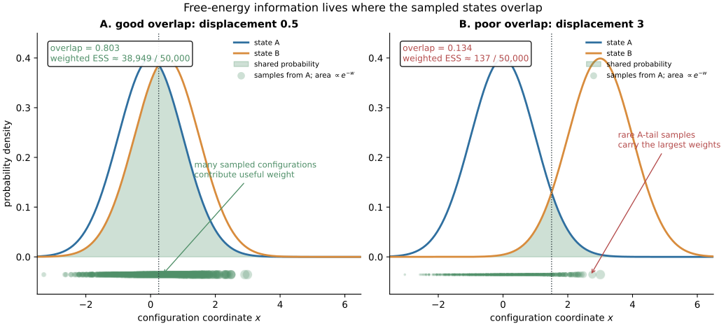
In the left panel, many ordinary A samples also look plausible under B, so the estimate averages many meaningful contributions. In the right panel, the B distribution is centered three standard deviations away. Only rare samples in the right tail of A carry substantial weight. Adding more typical A samples barely changes the estimate; reaching the rare tail matters much more.
The reported overlap coefficient is \(\int\min[p_A(x),p_B(x)]dx\) for this analytic control. Real molecular systems do not usually offer that integral. Work distributions, weight ESS, bidirectional consistency, and per-window overlap matrices are practical substitutes, but none is a universal proof of convergence.
BAR asks both directions where they agree
Reverse samples from state B define
\[w_R(\mathbf R)=u_A(\mathbf R)-u_B(\mathbf R).\]Forward FEP asks A to describe B; reverse FEP asks B to describe A. Their failures occur in opposite tails. BAR combines both samples and, for equal forward and reverse sample counts, solves
\[\frac{1}{N_A}\sum_{i=1}^{N_A} \frac{1}{1+e^{w_{F,i}-\Delta f}} = \frac{1}{N_B}\sum_{j=1}^{N_B} \frac{1}{1+e^{w_{R,j}+\Delta f}}.\]The sigmoid factors give the largest influence to work values near the candidate crossing, where the two states can both describe the configuration. The JAX code brackets the root and bisects it 80 times. For unequal sample counts, the equation requires the usual sample-count offset; the teaching function intentionally implements only the equal-count case used here.
BAR is statistically more efficient than choosing one FEP direction when both states have samples in their shared region (Bennett, 1976). It is not a machine for inventing overlap. When both simulations miss the connecting region, both sides of the equation are extrapolating from tails.
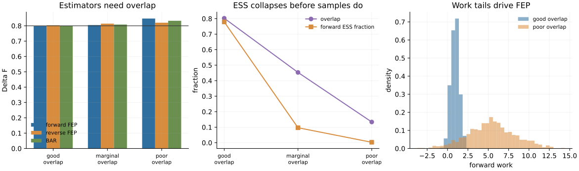
The independent full control quantifies the collapse:
| Control | Displacement | Overlap | Forward weighted ESS | Forward FEP | BAR | Exact |
|---|---|---|---|---|---|---|
| good | 0.5 | 0.803 | 38,949 / 50,000 | 0.7975 | 0.8004 | 0.8000 |
| marginal | 1.5 | 0.453 | 4,832 / 50,000 | 0.8046 | 0.8081 | 0.8000 |
| poor | 3.0 | 0.134 | 137 / 50,000 | 0.8472 | 0.8326 | 0.8000 |
The marginal FEP number is closer to the exact answer than its good-overlap counterpart in this one seeded run. Its ESS has nevertheless lost almost 90% of the nominal samples. Point-estimate luck is not a reliability diagnostic.
Where kUPS fits in the calculation
FEP and BAR do not replace molecular dynamics. They consume configurations that MD has sampled. A molecular workflow has three distinct layers:
- Sample: kUPS propagates atomic positions and momenta under state A, state B, or a set of biased intermediate states.
- Evaluate: the energy model evaluates both relevant reduced potentials on each stored configuration. JAX can vectorize these cross-state energy evaluations over frames.
- Estimate: the energy differences become forward and reverse work arrays, which the transparent JAX functions above reduce to \(\Delta f\) and diagnostics.
The Gaussian control skips layer 1 because independent normal samples have a known answer and isolate estimator behavior from integrator, thermostat, and MLIP errors. Calling those samples a kUPS simulation would weaken the test, not strengthen it.
Post 09 also avoids launching a redundant physical trajectory. Its real kUPS evidence is the three-replica 100 K argon run from Post 08. The configuration pins the execution summary, RDF-to-PMF summary, and compact curve by SHA-256; the workflow recomputes all three hashes before reading the data.
Python
smoke_dir = write_estimator_outputs(
    load_estimator_spec("09", "smoke"),
    output_root=Path("notebook-runs"),
)
fresh = load_estimator_summary(smoke_dir / "estimator_summary.json")
shared = fresh.shared_kups_evidence
dense, sparse = fresh.multistate_protocols or []
{
    "fresh profile": fresh.profile,
    "dense/sparse minimum overlap": (
        round(dense.min_adjacent_overlap, 3),
        round(sparse.min_adjacent_overlap, 3),
    ),
    "shared engine and device": (shared.engine, shared.observed_devices),
    "atoms x replicas x frames": (
        shared.atom_count,
        shared.replica_count,
        shared.frames_per_replica,
    ),
    "verified PMF source SHA-256": shared.pmf_curves_sha256,
}{'fresh profile': 'smoke',
'dense/sparse minimum overlap': (0.181, 0.0),
'shared engine and device': ('kups', ['gpu:NVIDIA RTX A5000']),
'atoms x replicas x frames': (256, 3, 80),
'verified PMF source SHA-256': 'a97aa33b0687d4113a317930e350af7197d5f68781bc722082d909a1627c6cb1'}The fresh smoke workflow confirms engine=kups, three 256-atom replicas with 80 frames each, and gpu:NVIDIA RTX A5000. It also verifies the complete PMF curve hash. This physical curve demonstrates support-sensitive free-energy analysis, but it is not presented as an FEP or BAR result. Post 10 performs the next missing step: actual biased kUPS umbrella trajectories connected by overlapping windows.
More states help only if they form a bridge
Suppose A and B are too different to overlap directly. Introduce intermediate states \(0,1,\ldots,K\) and sample each one. WHAM or MBAR can then combine the network rather than relying on one endpoint jump (Kumar et al., 1992; Shirts & Chodera, 2008).
The important object is a connected overlap graph:
\[0\longleftrightarrow1\longleftrightarrow2 \longleftrightarrow\cdots\longleftrightarrow K.\]Listing more windows does not guarantee that graph. If adjacent states 3 and 4 share no sampled configurations, the path is broken there. No estimator can determine the relative normalization of the two disconnected components from those samples alone.
The Post 09 multi-state control is intentionally a support-aware reconstruction, not production MBAR. Seven dense harmonic windows have minimum adjacent overlap 0.184 and no broken edges. Two endpoint-only windows have zero overlap, one broken edge, and a much larger support-aware PMF error. Its job is to make the connectivity failure falsifiable before Post 10 introduces WHAM-style analysis of biased kUPS trajectories.
Diagnose the configurations that control the answer
A defensible estimator report should answer more than “Which method did you use?”
| Question | Evidence to retain |
|---|---|
| What are A and B? | Hamiltonians, biases, temperature, and reduced-potential convention |
| Which configurations determine the estimate? | work distributions and the highest-weight frames |
| How concentrated are the weights? | directional weight ESS, reported with nominal sample count |
| Are the trajectories independently informative? | autocorrelation or block analysis in addition to weight ESS |
| Do both directions agree? | forward FEP, reverse FEP, and BAR where both samples exist |
| Is a multi-state path connected? | adjacent overlap matrix and an explicit broken-edge rule |
| Is the energy model valid there? | MLIP error or domain checks on high-leverage configurations |
| Can the calculation be reproduced? | configs, source revision, devices, seeds, and artifact hashes |
For an MLIP, the high-weight configurations deserve special attention. They are statistically influential precisely because they look unusual under the sampled state, which may also place them far from the model’s training domain. An estimator diagnostic and a model-validity diagnostic should therefore be evaluated on the same frames.
Check your understanding
- If one FEP configuration has work five units below another, how many times larger is its unnormalized weight?
- Why can 50,000 stored frames yield a weight ESS of only 137?
- If forward and reverse FEP disagree, what two distinct problems should you inspect?
- Can BAR recover a transition region visited by neither state?
- In a seven-window calculation, what does one zero-overlap adjacent pair do to the state network?
The first answer is \(e^5\approx148\). The remaining questions distinguish weight concentration, time correlation, state overlap, and graph connectivity.
The estimate is only as trustworthy as its shared configurations
FEP is an exact ratio written as an exponential average. BAR uses two directions to focus that comparison on their shared configurations. A chain of intermediate states can replace one impossible jump with several easier ones. All three statements have the same condition: the necessary configurations must actually have been sampled.
A free-energy number is therefore the end of the report, not the beginning. Show which configurations voted, how concentrated their weights were, whether the state network connected, and whether the potential was credible on the high-leverage frames. If those checks fail, redesign the sampling path rather than adding decimals to the estimate.
Reproducibility record and complete estimator dashboard
Run and verify the deterministic CPU control from the locked environment:
git clone https://github.com/sungsoo-ahn/kups-md-tutorials
cd kups-md-tutorials
uv sync --locked

uv run kups-tutorial run 09 --profile smoke
uv run kups-tutorial verify 09 --profile smoke
uv run kups-tutorial verify-notebooks --posts 09 --output-dir notebook-runs
uv run kups-tutorial export-notebook-cells \
  --executed-notebooks-dir notebook-runs \
  --site-root ../sungsoo-ahn.github.io --posts 09 --check
The estimator control does not require a GPU. Its shared physical evidence is accepted only when the pinned Post 08 summaries record real kUPS execution, observed GPU workers, raw-HDF5 hashes, and exact agreement with the copied PMF curve.
The complete audit dashboard retains FEP/BAR point estimates, overlap and ESS, work tails, connected and broken multi-state controls, and the shared physical kUPS PMF:
Source and evidence:
References
- Bennett, C. H. (1976). Efficient estimation of free energy differences from Monte Carlo data. Journal of Computational Physics, 22, 245–268. ↩
- Kumar, S., Rosenberg, J. M., Bouzida, D., Swendsen, R. H. & Kollman, P. A. (1992). The weighted histogram analysis method for free-energy calculations on biomolecules. Journal of Computational Chemistry, 13, 1011–1021. ↩
- Shirts, M. R. & Chodera, J. D. (2008). Statistically optimal analysis of samples from multiple equilibrium states. The Journal of Chemical Physics, 129, 124105. ↩