Free energy is the logarithm of probability. Common configurations have low free energy; rare configurations have high free energy. That sounds simple, but the logarithm makes the least sampled region of a histogram the most visually dramatic part of a free-energy curve.
If probability is underestimated by a factor of two, the free-energy error is \(k_{\mathrm B}T\log2\). If a bin is empty, its logarithm is not a measured high barrier. It is unsupported. Replacing zero by an arbitrary epsilon turns the epsilon—not the trajectory—into the barrier height.
We will expose that entire transformation. A short JAX implementation will build a weighted histogram, undo a sampling bias with the correct sign, mask empty bins, take the logarithm, and choose a relative reference. Then real kUPS pair separations will become an RDF and a supported pair potential of mean force (PMF).
- why relative free energy is a logarithm of probability;
- how bin width creates a bias–variance tradeoff before the logarithm;
- why biased samples receive weights \(\exp(+\beta V_b)\);
- why empty or low-probability bins must be reported as unsupported;
- how a raw radial probability differs from an RDF-based pair PMF;
- how support choices can dominate replica uncertainty.
Prerequisites: canonical sampling from Post 04, effective samples from Post 06, and RDF normalization from Post 07.
Probability determines relative free energy
Let \(s=s(\mathbf R)\) be a collective variable: a distance, angle, coordination, or other function of atomic positions. Its equilibrium probability density is
\[p(s) =\frac{1}{Z}\int d\mathbf R\, e^{-\beta U(\mathbf R)} \delta\!\left(s-s(\mathbf R)\right), \qquad \beta=\frac{1}{k_{\mathrm B}T}.\]The associated free-energy profile, or PMF along \(s\), is
\[F(s)=-k_{\mathrm B}T\log p(s)+C.\]The additive constant \(C\) is arbitrary because a normalized probability depends only on free-energy differences. This tutorial sets the minimum of each supported finite profile to zero. A reported barrier is then a difference between the supported basin and barrier regions, not an absolute energy.
The formula also implies an immediate uncertainty rule. For a small probability perturbation,
\[\delta F \approx -k_{\mathrm B}T\frac{\delta p}{p}.\]The same absolute probability error is therefore much more damaging where \(p\) is small. This is why smooth high-free-energy tails deserve more skepticism than well-populated minima.
A histogram is already a scientific choice
Given samples \(s_n\) and bins with widths \(\Delta s_b\), an unbiased density estimate is
\[\hat p_b =\frac{n_b}{N\,\Delta s_b}.\]Narrow bins resolve shape but contain fewer samples. Wide bins reduce counting noise but average over real curvature. More samples can reduce variance at a fixed bin width; they cannot remove discretization bias created by a bin that is too wide.
The full known-answer control draws 80,000 samples from
\[U(s)=(s^2-1)^2,\]whose minima are at \(s=\pm1\) and whose barrier at \(s=0\) is exactly one in reduced energy units:
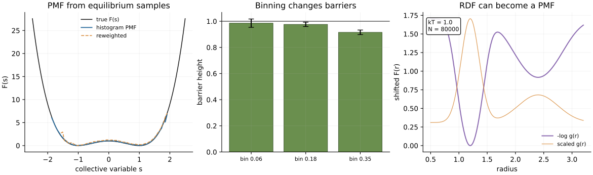
| Bin width | Estimated barrier | Bootstrap SE | Barrier error | Curve RMSE |
|---|---|---|---|---|
| 0.06 | 0.985 | 0.032 | -0.015 | 0.171 |
| 0.18 | 0.976 | 0.017 | -0.024 | 0.366 |
| 0.35 | 0.915 | 0.017 | -0.085 | 0.591 |
The coarsest histogram has the smallest displayed bootstrap error but the largest curve bias. Bootstrap resampling measures finite-sample variation of the chosen estimator. It does not discover that the estimator has smoothed away the barrier.
Implement weighted free energy in JAX
The collapsed setup selects a CPU backend and imports the real kUPS workflow.
Python
from pathlib import Path
import os

os.environ.setdefault("JAX_PLATFORMS", "cpu")

import jax
from jax import Array
import jax.numpy as jnp
from IPython.display import Image, display

from kups_md_tutorials.config import load_free_energy_spec
from kups_md_tutorials.free_energies import (
    load_kups_rdf_pmf_summary,
    write_free_energy_outputs,
)
from kups_md_tutorials.kups_engine import load_kups_result

repo_root = Path.cwd()
if not (repo_root / "configs").exists():
    repo_root = repo_root.parent
os.chdir(repo_root)
The open cell below implements the full probability-to-free-energy map. It accepts an optional bias energy for every sample. Subtracting the largest log weight before exponentiating improves numerical stability and does not change the normalized density. Empty bins remain NaN after the finite profile is shifted.
Python
def histogram_free_energy(
    samples: Array,
    bin_edges: Array,
    temperature: float,
    *,
    bias_values: Array | None = None,
    boltzmann_constant: float = 1.0,
) -> tuple[Array, Array, Array]:
    """Convert optionally biased samples into a shifted histogram free energy."""

    thermal_energy = boltzmann_constant * temperature
    log_weights = (
        jnp.zeros_like(samples)
        if bias_values is None
        else bias_values / thermal_energy
    )
    log_weights -= jnp.max(log_weights)
    weights = jnp.exp(log_weights)
    bin_weights, _ = jnp.histogram(samples, bins=bin_edges, weights=weights)

    bin_widths = bin_edges[1:] - bin_edges[:-1]
    probability_density = bin_weights / (jnp.sum(bin_weights) * bin_widths)
    supported = bin_weights > 0.0
    raw_free_energy = jnp.where(
        supported,
        -thermal_energy * jnp.log(probability_density),
        jnp.inf,
    )
    reference = jnp.min(raw_free_energy)
    shifted_free_energy = jnp.where(
        supported,
        raw_free_energy - reference,
        jnp.nan,
    )
    centers = 0.5 * (bin_edges[:-1] + bin_edges[1:])
    return centers, shifted_free_energy, supported


grid = jnp.linspace(-2.2, 2.2, 20_001)
true_energy = (grid**2 - 1.0) ** 2
samples = jax.random.choice(
    jax.random.PRNGKey(808), grid, shape=(80_000,), p=jax.nn.softmax(-true_energy)
)
centers, free_energy, supported = histogram_free_energy(
    samples, jnp.arange(-2.2, 2.21, 0.08), temperature=1.0
)
barrier = jnp.nanmin(free_energy[jnp.abs(centers) < 0.08])

two_state_samples = jnp.concatenate((jnp.zeros(20), jnp.ones(80)))
two_state_bias = jnp.where(two_state_samples == 0.0, jnp.log(4.0), 0.0)
_, two_state_free_energy, _ = histogram_free_energy(
    two_state_samples,
    jnp.array([-0.5, 0.5, 1.5]),
    temperature=1.0,
    bias_values=two_state_bias,
)
print(f"known barrier=1.000, estimated barrier={float(barrier):.3f}")
print(f"occupied bins={int(jnp.sum(supported))}/{supported.size}")
print(f"reweighted two-state free-energy difference={float(jnp.ptp(two_state_free_energy)):.2e}")known barrier=1.000, estimated barrier=1.005
occupied bins=50/55
reweighted two-state free-energy difference=0.00e+00
The JAX control estimates the known unit barrier as 1.005 from 80,000 samples. Fifty of 55 bins are occupied; the other five are visibly unsupported rather than assigned a numerical wall.
The two-state sanity check is more important than it looks. The observed sample counts are 20 versus 80 because the first state carries a positive bias \(V_b=\log4\) in reduced units. Multiplying its samples by \(e^{+V_b}=4\) restores equal target weights and a free-energy difference of zero to machine precision. A negative reweighting sign would amplify the bias instead of removing it.
Reweighting removes a known bias, not missing configurations
Suppose a simulation samples a biased energy \(U(\mathbf R)+V_b(s)\). Its collective-variable density is
\[p_b(s)\propto e^{-\beta[F(s)+V_b(s)]}.\]Solving for the unbiased density gives the sample weight
\[w(s)=e^{+\beta V_b(s)}.\]The positive sign cancels the negative bias factor already present in the sampled distribution. For numerical work, one should accumulate these weights with shifted log weights or a log-sum-exp formulation.
Reweighting cannot create support. If no biased sample visits a region, its unbiased probability remains unknown. If a few enormous weights dominate, the effective sample size collapses even if the raw sample count is large. The full double-well bias control recovers a barrier of 1.123; its remaining 0.123 error is a finite-overlap and sampling limitation, not a reason to adjust the sign (Torrie & Valleau, 1977).
A radial histogram and a pair PMF are not the same object
For a homogeneous isotropic system, the probability of observing a pair separation in \([r,r+dr]\) contains a geometric shell factor:
\[p_{\mathrm{pair}}(r)\,dr \propto 4\pi r^2\rho\,g(r)\,dr.\]Taking \(-k_{\mathrm B}T\log p_{\mathrm{pair}}(r)\) directly would include the radial Jacobian \(r^2\). The RDF defined in Post 07 has already divided out that ideal-gas shell measure. Its pair PMF is therefore
\[W(r)=-k_{\mathrm B}T\log g(r)+C.\]These are two different free-energy conventions. One describes probability in the scalar coordinate \(r\), including how shell volume grows. The other describes pair correlations relative to an ideal gas. A plot must name which object it shows.
The pair PMF is also not the bare pair potential. It is a many-body equilibrium quantity for a chosen temperature, density, composition, and ensemble. At low density it may approach the pair potential more closely; that is not assumed for this finite-density tutorial.
Transform new kUPS RDF samples carefully
The physical workflow runs three fixed-volume Lennard-Jones argon replicas at 100 K. Each uses kUPS baoab_langevin with a 2 fs step and stores a frame every 20 fs. The analysis:
- reads positions and volume from each HDF5 trajectory;
- applies the periodic RDF estimator from Post 07;
- averages the RDF across independent replicas;
- masks bins whose mean \(g(r)\) is below a declared threshold;
- applies \(-k_{\mathrm B}T\log g(r)\) and shifts the supported minimum;
- transforms each replica separately to obtain a PMF spread.
The next cell launches two fresh 32-atom CPU smoke replicas and reports every support rule alongside the primary result.
Python
smoke_dir = write_free_energy_outputs(
    load_free_energy_spec("08", "smoke"),
    output_root=Path("notebook-runs"),
)
physical = load_kups_rdf_pmf_summary(smoke_dir / "kups_rdf_pmf_summary.json")
execution = load_kups_result(smoke_dir / "kups_md_summary.json")
{
    "engine": physical.engine,
    "devices": [case.observed_devices for case in execution.cases],
    "atoms x replicas x frames": (
        physical.atom_count, physical.replica_count, physical.frames_per_replica
    ),
    "PMF minimum radius (angstrom)": round(physical.pmf_minimum_radius_angstrom, 2),
    "PMF range (meV)": round(1000 * physical.pmf_range_ev, 1),
    "support thresholds": physical.support_thresholds,
    "threshold ranges (meV)": tuple(
        round(1000 * value, 1) for value in physical.support_threshold_pmf_ranges_ev
    ),
    "max replica std (meV)": round(
        1000 * physical.max_replica_pmf_standard_deviation_ev, 1
    ),
}{'engine': 'kups',
'devices': [['cpu:cpu'], ['cpu:cpu']],
'atoms x replicas x frames': (32, 2, 16),
'PMF minimum radius (angstrom)': 3.75,
'PMF range (meV)': 28.1,
'support thresholds': (0.02, 0.05, 0.1),
'threshold ranges (meV)': (40.3, 28.1, 28.1),
'max replica std (meV)': 5.6}The smoke profile places its PMF minimum at 3.75 Å. Under \(g(r)\ge0.05\), its range is 28.1 meV; changing the threshold to 0.02 expands the range to 40.3 meV. The maximum replica standard deviation is 5.6 meV. Sixteen frames per replica make these execution diagnostics, not a converged pair PMF.
The full profile has three 256-atom replicas, 200 warmup steps, 80 stored frames per replica, and an 8.0 Å range below the 10.52 Å half-box support. Every worker observed an NVIDIA RTX A5000:
| Replica | Frames | Mean temperature | Runtime | HDF5 SHA-256 prefix | Device |
|---|---|---|---|---|---|
| 0 | 80 | 100.48 K | 53.40 s | 07d605fcf78f | RTX A5000 |
| 1 | 80 | 98.84 K | 50.17 s | e4a1d621418a | RTX A5000 |
| 2 | 80 | 99.40 K | 50.76 s | 942f4c0281ed | RTX A5000 |
At 100 K, \(k_{\mathrm B}T=8.62\) meV. The mean RDF peak is 4.679 at 3.64 Å, so the shifted pair PMF minimum occurs at the same radius. Under the primary \(g(r)\ge0.05\) rule, 60 radial bins remain finite and the PMF spans 37.98 meV, or about \(4.4k_{\mathrm B}T\).
Watch pair occupancy invert into pair free energy
The left panel below follows minimum-image displacements from atom 0 to nearby atoms in 20 stored frames of full replica 0. Orange points have three-dimensional distances in the 3.2–4.2 Å first-shell range. Their projections accumulate near the radius of the first RDF peak.
The right panel uses the complete three-replica RDF, not the selected atom cloud. Blue shows \(g(r)\); orange shows the supported shifted PMF. A high RDF peak becomes a PMF minimum because the logarithm reverses occupancy.
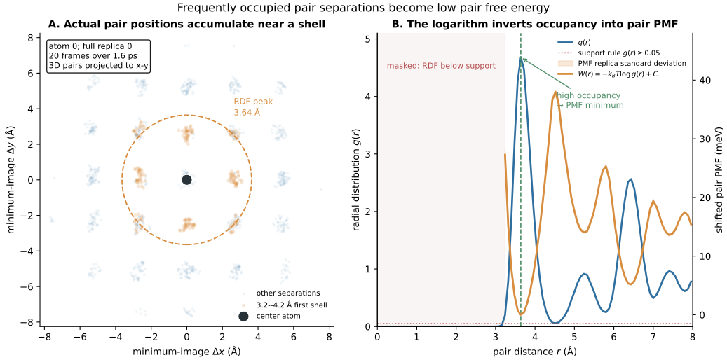
The atom cloud supplies physical intuition, not the final probability estimate. It uses one center atom and one replica; the RDF and PMF pool all pairs and frames across three replicas. Keeping those evidence levels distinct prevents an appealing configuration from standing in for a sampled distribution.
The support threshold can dominate the error budget
The full PMF has a maximum between-replica standard deviation of only 0.85 meV. That looks precise until the low-RDF support rule changes:
| Minimum supported \(g(r)\) | Finite bins | Shifted PMF range | PMF minimum |
|---|---|---|---|
| 0.02 | 61 | 45.50 meV | 3.64 Å |
| 0.05 | 60 | 37.98 meV | 3.64 Å |
| 0.10 | 57 | 31.27 meV | 3.64 Å |
The support choice changes the displayed range by 14.24 meV—far more than the replica band—while leaving the minimum location stable. This is a useful partial result: the preferred first-shell separation is robust under these rules, but the high-PMF range is not.
Replica agreement cannot diagnose a shared analysis choice. All replicas can agree in a low-probability region where the logarithm is nevertheless driven by a threshold, pseudocount, or bin width. Estimator sensitivity and sampling uncertainty must be reported separately.
What would make a free-energy claim defensible?
A free-energy profile should report:
- the collective variable and its Jacobian convention;
- ensemble, temperature, and any sampling bias;
- histogram or density estimator and all bandwidth parameters;
- reweighting equation, sign, numerical stabilization, and weight ESS;
- empty-bin and low-support policy;
- arbitrary reference shift;
- replica, block, and estimator-sensitivity uncertainties;
- evidence that every interpreted basin and barrier was sampled.
The current full run validates the transform and exposes support sensitivity. It does not establish a converged argon pair PMF. A production study would need longer warmup and trajectories, more replicas, RDF-bin sensitivity, finite-size checks, and a state-point-specific physical interpretation (Frenkel & Smit, 2001).
For rare collective-variable transitions, ordinary trajectories may never visit the barrier often enough. Posts 09 and 10 will introduce free-energy estimators and umbrella sampling designed around overlap between biased states.
Check your understanding
- If a probability is underestimated by a factor of two, by how much is its free energy overestimated?
- Why does a small bootstrap error at one fixed bin width not prove that the free-energy curve has low bias?
- What sign must appear in the weight that removes an added bias \(V_b(s)\), and why?
- Why is \(-k_{\mathrm B}T\log p_{\mathrm{pair}}(r)\) different from \(-k_{\mathrm B}T\log g(r)\)?
The first answer is \(k_{\mathrm B}T\log2\). The others distinguish estimator bias, bias removal, and the radial Jacobian from ordinary sampling noise.
A free-energy curve is only as strong as its least-supported claim
The logarithm converts occupancy into a relative energy landscape. It also magnifies every weakness in rare bins. A correct analysis keeps unsupported regions missing, exposes its bias weights and reference shift, and compares sampling uncertainty with estimator sensitivity.
The deepest minimum is usually the easiest part to estimate. The tempting high barrier at the edge of support is often the least trustworthy. A free-energy plot becomes evidence only when its probability support remains visible.
Reproducibility record and complete free-energy dashboard
Run and verify the CPU profile from the locked environment:
git clone https://github.com/sungsoo-ahn/kups-md-tutorials
cd kups-md-tutorials
uv sync --locked

uv run kups-tutorial run 08 --profile smoke
uv run kups-tutorial verify 08 --profile smoke
uv run kups-tutorial verify-notebooks --posts 08 --output-dir notebook-runs
uv run kups-tutorial export-notebook-cells \
  --executed-notebooks-dir notebook-runs \
  --site-root ../sungsoo-ahn.github.io --posts 08 --check
The complete audit dashboard retains double-well bin-width controls, bootstrap error, biased-sample reweighting, a synthetic RDF check, the real kUPS pair PMF, replica band, and all three support thresholds:
Source and evidence: