An MD trajectory is a sequence of microscopic states. It stores where atoms were and how they moved. It does not contain a radial distribution function, coordination number, or diffusion coefficient waiting in a column. Those quantities appear only after an estimator turns the stored state into a measurement.
That distinction matters because almost any trajectory can produce a smooth curve. A raw distance histogram can resemble an RDF while missing the shell volume and density normalization. A velocity-correlation tail can look stable even when only a few time origins support it. Plotting is the last step, not the validation.
We will make the estimator visible. First, a short JAX function will apply minimum-image geometry, count unordered pairs, normalize spherical shells, and integrate coordination. Then the same operations will be applied to real kUPS HDF5 positions, while momenta and masses provide a velocity autocorrelation.
- how a microscopic trajectory becomes a macroscopic estimator;
- how periodic minimum-image distances enter an RDF;
- why pair counts must be divided by shell volume, density, frames, and pair convention;
- how coordination is an integral with a user-chosen cutoff;
- how velocity autocorrelation uses many overlapping time origins;
- how support limits and replica uncertainty constrain every curve.
Prerequisites: periodic cells from the foundations lesson, real HDF5 state from Post 01, and observable-specific effective samples from Post 06.
An observable is a rule applied to state
At stored frame \(t\), let the atom positions be \(\mathbf R_t=(\mathbf r_{1,t},\ldots,\mathbf r_{N,t})\) and momenta be \(\mathbf P_t\). A scalar observable is a function of that state:
\[A_t=A(\mathbf R_t,\mathbf P_t,\mathbf h_t),\]where \(\mathbf h_t\) is the periodic cell. An equilibrium average estimates an ensemble expectation by averaging the time series,
\[\langle A\rangle \approx \frac{1}{N_f}\sum_{t=0}^{N_f-1} A_t.\]The function \(A\) is the scientific definition. It specifies geometry, normalization, units, parameters, and valid support. The average adds sampling assumptions: warmup, correlation, and replica coverage. Two groups can analyze the same HDF5 file and obtain different “coordination numbers” simply because they used different cutoffs.
This chapter uses two kinds of observable:
- structural: the RDF and its coordination integral depend on positions;
- dynamical: the velocity autocorrelation depends on momenta at separated times.
The first asks how atoms are arranged. The second asks how motion remembers itself.
Start from periodic pair displacement
For atoms \(i\) and \(j\) in a cubic cell of length \(L\), the raw displacement is \(\Delta\mathbf r_{ij}=\mathbf r_i-\mathbf r_j\). Periodic copies make that vector ambiguous. The minimum-image convention chooses the nearest copy:
\[\Delta\mathbf r_{ij}^{\mathrm{MIC}} = \Delta\mathbf r_{ij} -L\operatorname{round}\!\left(\frac{\Delta\mathbf r_{ij}}{L}\right).\]The pair distance is its norm. This componentwise expression is appropriate for the cubic cells used here. General triclinic cells are handled more safely through fractional coordinates and the complete cell matrix.
We count each unordered pair once, so only indices \(i<j\) enter the histogram. Counting both \((i,j)\) and \((j,i)\) is also valid, but the expected count must then change by a factor of two.
Periodic boundaries do not grant unlimited radial support. Under this cubic minimum-image estimator, a complete spherical shell must satisfy
\[r \le \frac{L}{2}.\]Beyond half the box, corners of the nominal shell cannot be represented uniformly by minimum images. Drawing an RDF line there does not create the missing pair geometry.
Pair counts become an RDF only after normalization
Let radial bin \(b\) span \([r_b,r_{b+1})\). Its exact spherical-shell volume is
\[\Delta V_b =\frac{4\pi}{3}\left(r_{b+1}^3-r_b^3\right).\]For \(N\) atoms, number density \(\rho=N/V\), \(N_f\) frames, and unordered pairs, an ideal-gas reference contributes the expected count
\[n_b^{\mathrm{ideal}} =\frac{1}{2}N_fN\rho\,\Delta V_b.\]The RDF estimator is therefore
\[g_b=\frac{n_b}{n_b^{\mathrm{ideal}}}.\]The shell volume removes the geometric growth of available space with radius. The density makes systems comparable, the frame count converts accumulated counts to a per-frame estimate, and the factor one-half matches the unordered pair convention. In a spatially uniform ideal gas, \(g(r)\rightarrow1\) away from finite-size and sampling noise (Allen & Tildesley, 1987).
Implement periodic RDF and coordination in JAX
The collapsed setup selects the CPU backend, imports the known FCC system, and loads the real kUPS workflow.
Python
from pathlib import Path
import os

os.environ.setdefault("JAX_PLATFORMS", "cpu")

from jax import Array
import jax.numpy as jnp
from IPython.display import Image, display

from kups_md_tutorials.config import load_observable_spec
from kups_md_tutorials.kups_engine import load_kups_result
from kups_md_tutorials.observables import (
    load_kups_observable_summary,
    write_observable_outputs,
)
from kups_md_tutorials.systems import argon_fcc

repo_root = Path.cwd()
if not (repo_root / "configs").exists():
    repo_root = repo_root.parent
os.chdir(repo_root)
The open cell below performs every central operation. Broadcasting constructs all frame/atom/atom displacements, round applies the minimum image, triu keeps each pair once, and histogram counts radial bins. Unsupported bins are set to NaN instead of being silently plotted.
Python
def periodic_rdf_and_coordination(
    positions: Array,
    box_length: float,
    bin_edges: Array,
    *,
    coordination_cutoff: float,
) -> tuple[Array, Array, Array, Array]:
    """Estimate an RDF and coordination from cubic periodic trajectory frames."""

    frame_count, atom_count, _ = positions.shape
    displacement = positions[:, :, None, :] - positions[:, None, :, :]
    displacement -= box_length * jnp.round(displacement / box_length)
    distance = jnp.linalg.norm(displacement, axis=-1)

    unordered_pair = jnp.triu(jnp.ones((atom_count, atom_count), dtype=bool), k=1)
    pair_distances = jnp.where(unordered_pair[None, :, :], distance, jnp.inf)
    counts, _ = jnp.histogram(pair_distances.reshape(-1), bins=bin_edges)

    radii = 0.5 * (bin_edges[:-1] + bin_edges[1:])
    shell_volumes = (4.0 * jnp.pi / 3.0) * (
        bin_edges[1:] ** 3 - bin_edges[:-1] ** 3
    )
    number_density = atom_count / box_length**3
    expected_counts = (
        0.5 * frame_count * atom_count * number_density * shell_volumes
    )
    supported = bin_edges[1:] <= 0.5 * box_length
    rdf = jnp.where(supported, counts / expected_counts, jnp.nan)

    inside_cutoff = supported & (bin_edges[1:] <= coordination_cutoff)
    coordination = number_density * jnp.sum(
        jnp.where(inside_cutoff, rdf * shell_volumes, 0.0)
    )
    return radii, rdf, supported, coordination


fcc = argon_fcc(2, 0.0275)
box_length = float(fcc.cell.lengths()[0])
radii, rdf, supported, coordination = periodic_rdf_and_coordination(
    jnp.asarray(fcc.positions)[None, :, :],
    box_length,
    jnp.arange(0.0, 8.08, 0.08),
    coordination_cutoff=5.12,
)
peak = int(jnp.nanargmax(rdf))
print(f"atoms={len(fcc)}, box length={box_length:.2f} Å")
print(f"first RDF peak={float(radii[peak]):.2f} Å")
print(f"coordination through 5.12 Å={float(coordination):.1f}")
print(f"last supported bin center={float(radii[supported][-1]):.2f} Å")atoms=32, box length=10.52 Å
first RDF peak=3.72 Å
coordination through 5.12 Å=12.0
last supported bin center=5.16 Å
The control is one exact 32-atom FCC frame at the same density as the physical runs. Its first pair shell appears at 3.72 Å. Integrating through 5.12 Å returns exactly 12 neighbors, the FCC nearest-neighbor count. The last fully supported bin center is 5.16 Å because the half-box boundary lies at 5.26 Å.
The coordination calculation uses the same shell volumes as the RDF:
\[n_c(r_c) =4\pi\rho\int_0^{r_c}r^2g(r)\,dr \approx \rho\sum_{r_{b+1}\le r_c}g_b\Delta V_b.\]The cutoff \(r_c\) is part of the observable. It is usually placed at a physically motivated minimum after the first RDF peak. Moving it into the next shell changes the reported coordination even when no trajectory frame changes.
The transparent JAX function assumes a fixed cubic cell. The production analysis reads the stored volume and uses the same pair and shell convention; a moving or noncubic cell would require per-frame cell geometry.
Run the estimators on new kUPS trajectories
The physical workflow runs Lennard-Jones argon at 100 K and fixed volume. Each replica uses the kUPS baoab_langevin path with a 2 fs timestep and an independent momentum seed. One frame is stored every ten steps, or 20 fs.
The analysis reads rather than invents its microscopic inputs:
- positions for minimum-image pair distances;
- volume for density and radial support;
- momenta and per-atom masses for velocities;
- replica identity for between-run uncertainty.
The next cell launches two fresh 32-atom CPU smoke replicas through kups.application.simulations.md.run and analyzes their HDF5 files.
Python
smoke_dir = write_observable_outputs(
    load_observable_spec("07", "smoke"),
    output_root=Path("notebook-runs"),
)
physical = load_kups_observable_summary(smoke_dir / "kups_observable_summary.json")
execution = load_kups_result(smoke_dir / "kups_md_summary.json")
{
    "engine": physical.engine,
    "devices": [case.observed_devices for case in execution.cases],
    "atoms x replicas x frames": (
        physical.atom_count, physical.replica_count, physical.frames_per_replica
    ),
    "RDF first peak": (
        round(physical.rdf_first_peak_radius_angstrom, 2),
        round(physical.rdf_first_peak_value, 2),
    ),
    "coordination +/- replica SE": (
        round(physical.coordination_number, 2),
        round(physical.coordination_replica_standard_error, 3),
    ),
    "VACF integral (fs)": round(physical.vacf_integral_fs, 1),
}{'engine': 'kups',
'devices': [['cpu:cpu'], ['cpu:cpu']],
'atoms x replicas x frames': (32, 2, 16),
'RDF first peak': (3.75, 4.99),
'coordination +/- replica SE': (12.6, 0.076),
'VACF integral (fs)': 42.1}The smoke output has 16 frames per replica. It places the first RDF peak at 3.75 Å with height 4.99, estimates coordination as \(12.60\pm0.08\) by replica standard error, and obtains a 42.1 fs normalized VACF integral. These short-run values prove the code path; they are not production estimates.
The full profile uses three independent 256-atom replicas and 80 frames per replica. Its requested 8.0 Å RDF range is below the 10.52 Å half-box support. Every worker observed an NVIDIA RTX A5000:
| Replica | Frames | Mean temperature | Runtime | HDF5 SHA-256 prefix | Device |
|---|---|---|---|---|---|
| 0 | 80 | 99.89 K | 53.43 s | 3aa322ef0943 | RTX A5000 |
| 1 | 80 | 98.45 K | 50.00 s | d065bbd2cda2 | RTX A5000 |
| 2 | 80 | 102.23 K | 50.46 s | 342396071b71 | RTX A5000 |
Distinct seeds and HDF5 hashes establish separate executions. They do not by themselves prove that every slow physical mode was sampled independently.
See one neighbor shell become the RDF
The left panel below selects atom 0 in the final frame of full replica 0 and places it at the origin. Every displayed displacement uses the periodic minimum image. Orange atoms lie inside the three-dimensional 5.1 Å coordination sphere; pale atoms are outside the cutoff but inside the 8 Å RDF range. Marker size encodes the magnitude of the hidden \(z\) displacement.
The right panel then replaces this single neighborhood with all unordered pairs from all frames and replicas. Shell normalization produces the RDF, and the green cutoff selects the bins used by the coordination integral.
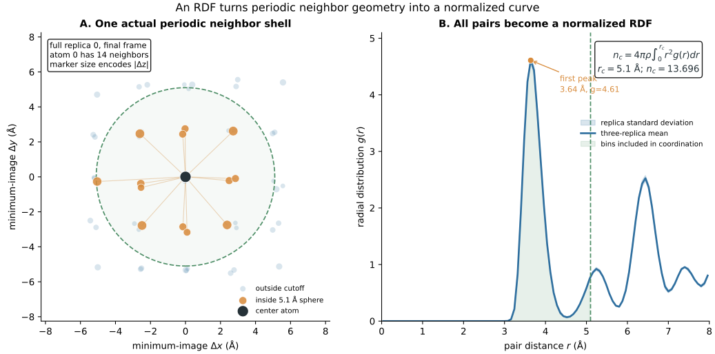
The distinction between 14 and 13.696 is important. The first is one atom in one frame. The second averages a defined RDF estimator over all atoms, 80 frames, and three replicas. An atom-level picture builds intuition, but the reported scalar needs the complete estimator and sampling record.
Across replicas, full coordination ranges from 13.678 to 13.722, giving a replica standard error of 0.013. It is not a universal argon coordination. It belongs to this potential, density, temperature, warmup, cutoff, bin width, and 1.6 ps stored window.
Velocity memory is another trajectory estimator
Positions describe structure. Dynamics require time ordering. kUPS stores momenta \(\mathbf p_{i,t}\) and masses \(m_i\), so velocities are
\[\mathbf v_{i,t}=\frac{\mathbf p_{i,t}}{m_i}.\]For lag \(k\), the normalized velocity autocorrelation function (VACF) averages over atoms and all time origins that still have a partner:
\[C_v(k) = \frac{ \dfrac{1}{N\,(N_f-k)}\sum_{t=0}^{N_f-k-1}\sum_i \mathbf v_{i,t}\cdot\mathbf v_{i,t+k} }{ \dfrac{1}{N\,N_f}\sum_{t=0}^{N_f-1}\sum_i \mathbf v_{i,t}\cdot\mathbf v_{i,t} }.\]The numerator has fewer time origins as \(k\) grows. Long-lag noise therefore increases even before physical finite-size effects enter. Replica bands and a reported maximum lag are part of the estimator, not cosmetic additions.
The full mean VACF is 0.799 at the first 20 fs lag and first crosses zero near 140 fs. Its displayed 0–600 fs integral is \(7.06\pm0.33\) fs by replica standard error.
That integral is not a diffusion coefficient. For an isotropic fluid, the Green–Kubo relation uses the unnormalized velocity correlation:
\[D =\frac{1}{3}\int_0^\infty \left\langle\mathbf v(0)\cdot\mathbf v(t)\right\rangle dt =\frac{\langle v^2\rangle}{3}\int_0^\infty C_v(t)\,dt.\]This tutorial has a coarse 20 fs storage interval, a short tail, and no hydrodynamic finite-size correction. It therefore reports the normalized integral only as a dynamical-memory diagnostic (Kubo, 1957).
Every curve needs support and uncertainty
An error bar on coordination does not quantify the entire RDF. RDF bins share atoms and frames, and VACF lags share time origins. The full analysis therefore records the mean and between-replica standard deviation at every RDF bin and VACF lag. The maximum replica standard deviation is 0.077 for the RDF and 0.0088 for the normalized VACF.
Replica spread and within-run correlation answer different questions. Blocks probe finite-time memory inside one run. Independent replicas expose trajectory-to-trajectory disagreement. A serious observable study often needs both, especially if metastability makes one long trajectory deceptively smooth (Frenkel & Smit, 2001).
Before accepting a trajectory-derived observable, record:
- microscopic inputs and their units;
- pair, normalization, and time-origin conventions;
- bin width, cutoff, and maximum lag;
- periodic-cell support and finite-size assumptions;
- warmup, storage interval, effective samples, and replica spread;
- sensitivity to analysis parameters and trajectory extension.
The bounded full run demonstrates this measurement contract and a real GPU kUPS path. It does not establish converged liquid structure, a transport coefficient, or force-model validity.
Check your understanding
- If ordered pairs are counted instead of unordered pairs, which factor in the ideal reference count must change?
- Why does a raw pair histogram grow with radius even in a uniform gas?
- Can two coordination numbers computed from the same RDF disagree without either implementation being numerically wrong?
- Why are the last VACF lags noisier than the first even before considering slow physics?
The answers follow from estimator definitions: ordered pairs double the count, spherical shells grow as \(r^2\), coordination depends on its cutoff, and long lags have fewer time origins.
A plot becomes a result only after its estimator is explicit
Positions do not become an RDF until periodic pair geometry is normalized against shell volume and density. An RDF does not become coordination until a cutoff and quadrature are chosen. Momenta do not become a transport result until velocities, time origins, tail support, and Green–Kubo normalization are specified.
A reproducible observable reports that entire path from microscopic arrays to the final quantity. Post 08 will invert a different measured object—a probability distribution—to obtain relative free energy.
Reproducibility record and complete observable dashboard
Run and verify the CPU profile from the locked environment:
git clone https://github.com/sungsoo-ahn/kups-md-tutorials
cd kups-md-tutorials
uv sync --locked

uv run kups-tutorial run 07 --profile smoke
uv run kups-tutorial verify 07 --profile smoke
uv run kups-tutorial verify-notebooks --posts 07 --output-dir notebook-runs
uv run kups-tutorial export-notebook-cells \
  --executed-notebooks-dir notebook-runs \
  --site-root ../sungsoo-ahn.github.io --posts 07 --check
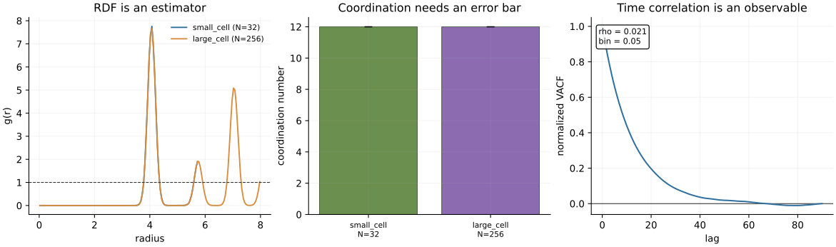
The complete audit dashboard retains the known FCC estimator controls, finite-size support check, block uncertainty, full VACF, and full RDF with replica bands:
Source and evidence:
References
- Allen, M. P. & Tildesley, D. J. (1987). Computer Simulation of Liquids. Oxford University Press. ↩
- Kubo, R. (1957). Statistical-mechanical theory of irreversible processes. I. Journal of the Physical Society of Japan, 12, 570–586. ↩
- Frenkel, D. & Smit, B. (2001). Understanding Molecular Simulation: From Algorithms to Applications. Academic Press. ↩