A saved MD frame is not a new experiment. It is the next state of the same trajectory. Positions have moved only a little, velocities retain memory, and collective structures may remain unchanged for much longer. Saving ten times more often can therefore make a file ten times larger without adding ten times more information.
That is why “we ran one million steps” is not a precision statement. To decide whether a trajectory supports a reported average, we need to separate three failures:
- initial-condition bias: early frames still remember how the system was prepared;
- temporal correlation: retained frames are not independent draws;
- replica disagreement: one trajectory may remain in a region that other independent runs visit differently.
This chapter turns those ideas into an explicit JAX estimator, runs independent kUPS trajectories, and follows actual atoms through their stored frames. The answer will not be a universal step count. It will be an observable-specific effective sample count and uncertainty target.
- why MD frames are time-correlated samples rather than independent data;
- how to compute a normalized autocorrelation function and integrated autocorrelation time;
- how raw frame count becomes an effective sample size;
- why warmup, within-run correlation, and independent replicas diagnose different problems;
- how to define “long enough” relative to an observable and error tolerance.
Prerequisites: trajectories and saved state from the foundations lesson, thermostatted dynamics from Post 04, and the distinction between response and equilibration from Post 05.
A trajectory is a correlated time series
Let \(A_t\) be an observable evaluated at stored frame \(t\). It could be potential energy per atom, coordination number, density, or a molecular distance. From \(N\) retained frames, its sample mean is
\[\bar A = \frac{1}{N}\sum_{t=0}^{N-1} A_t.\]If the frames were independent, the familiar standard error would be \(s_A/\sqrt{N}\). MD violates that assumption. A particle at frame \(t+1\) starts from the position and momentum at frame \(t\), so nearby observable values tend to move together.
The normalized lag-\(k\) autocorrelation estimates that memory:
\[\rho_k = \frac{ \sum_{t=0}^{N-k-1}(A_t-\bar A)(A_{t+k}-\bar A) }{ \sum_{t=0}^{N-1}(A_t-\bar A)^2 }.\]At zero lag, \(\rho_0=1\). If \(\rho_1\) is close to one, a frame and its immediate successor contain strongly overlapping information. As the lag grows, memory usually decays, although finite trajectories make the tail noisy.
The integrated autocorrelation time used in this tutorial is
\[\tau_{\mathrm{int}} = 1 + 2\sum_{k=1}^{K}\rho_k,\]where \(K\) stops at the first nonpositive correlation. This simple positive-sequence window prevents a noisy long-lag tail from dominating the sum. Other window rules exist, so a reported autocorrelation time should always state its convention (Sokal, 1997).
Our convention measures \(\tau_{\mathrm{int}}\) in stored frames. The corresponding effective sample size is
\[N_{\mathrm{eff}} = \frac{N}{\tau_{\mathrm{int}}}, \qquad \operatorname{SE}_{\mathrm{corr}}(\bar A) \approx \frac{s_A}{\sqrt{N_{\mathrm{eff}}}}.\]Correlation therefore enlarges the naive error bar by approximately \(\sqrt{\tau_{\mathrm{int}}}\). It does not change how many frames are stored; it changes how much independent information those frames carry.
Compute the estimator in JAX
The collapsed setup selects a CPU backend and imports the real kUPS runner.
Python
from pathlib import Path
import os

os.environ.setdefault("JAX_PLATFORMS", "cpu")

import jax
from jax import Array
import jax.numpy as jnp
from IPython.display import Image, display

from kups_md_tutorials.config import load_trajectory_length_spec
from kups_md_tutorials.kups_engine import load_kups_result
from kups_md_tutorials.trajectory_length import (
    load_kups_trajectory_length_summary,
    write_trajectory_length_outputs,
)

repo_root = Path.cwd()
if not (repo_root / "configs").exists():
    repo_root = repo_root.parent
os.chdir(repo_root)
The open cell below implements the equations directly. jnp.correlate forms all lagged dot products; a cumulative positive mask stops the integrated sum at the first nonpositive value. No tutorial summary is loaded to obtain the answer.
Python
def autocorrelation_and_effective_sample_size(
    values: Array,
    *,
    max_lag: int = 100,
) -> tuple[Array, Array, Array]:
    """Estimate a positive-sequence autocorrelation time and sample count."""

    centered = values - jnp.mean(values)
    denominator = jnp.dot(centered, centered)
    lag_limit = min(max_lag, values.shape[0] - 1)
    full_correlation = jnp.correlate(centered, centered, mode="full")
    numerators = full_correlation[
        values.shape[0] - 1 : values.shape[0] + lag_limit
    ]
    correlation = numerators / jnp.where(denominator > 0.0, denominator, 1.0)
    constant_series = jnp.concatenate(
        (jnp.ones(1, dtype=values.dtype), jnp.zeros(lag_limit, dtype=values.dtype))
    )
    correlation = jnp.where(denominator > 0.0, correlation, constant_series)

    positive_prefix = jnp.cumprod((correlation[1:] > 0.0).astype(values.dtype))
    integrated_time = jnp.maximum(
        1.0,
        1.0 + 2.0 * jnp.sum(correlation[1:] * positive_prefix),
    )
    effective_samples = values.shape[0] / integrated_time
    return correlation, integrated_time, effective_samples


phi = 0.9
noise = jax.random.normal(jax.random.PRNGKey(606), (6_000,))
_, correlated = jax.lax.scan(
    lambda previous, xi: (
        phi * previous + jnp.sqrt(1.0 - phi**2) * xi,
        phi * previous + jnp.sqrt(1.0 - phi**2) * xi,
    ),
    0.0,
    noise,
)
correlated = correlated[1_000:]
correlation, tau_int, n_eff = autocorrelation_and_effective_sample_size(
    correlated, max_lag=200
)
naive_se = jnp.std(correlated, ddof=1) / jnp.sqrt(correlated.size)
corrected_se = jnp.std(correlated, ddof=1) / jnp.sqrt(n_eff)
print(f"analytic tau_int={(1 + phi) / (1 - phi):.1f}")
print(f"estimated tau_int={float(tau_int):.2f}")
print(f"raw samples={correlated.size}, effective samples={float(n_eff):.1f}")
print(f"naive SE={float(naive_se):.4f}, correlation-aware SE={float(corrected_se):.4f}")analytic tau_int=19.0
estimated tau_int=21.88
raw samples=5000, effective samples=228.6
naive SE=0.0147, correlation-aware SE=0.0687
The control is an autoregressive process,
\[X_{t+1}=\phi X_t + \sqrt{1-\phi^2}\,\xi_t, \qquad \xi_t\sim\mathcal N(0,1).\]For \(\phi=0.9\), its exact correlation is \(\rho_k=\phi^k\) and its infinite-run integrated time is
\[\tau_{\mathrm{int}} =1+2\sum_{k=1}^{\infty}\phi^k =\frac{1+\phi}{1-\phi} =19.\]The finite JAX realization estimates 21.88. Its 5,000 retained values become only 228.6 effective samples. The naive standard error is 0.0147; accounting for correlation raises it to 0.0687. The estimate is not supposed to equal 19 exactly: autocorrelation itself is estimated from finite correlated data.
This is a deliberately simple estimator. Near a phase transition or in a multimodal system, the first-zero window can miss a slow positive tail. A production analysis should compare window choices, block estimates, trajectory lengths, and independent replicas rather than treating one ESS number as a certificate.
Warmup removes bias, not correlation
Autocorrelation analysis assumes that the retained time series is reasonably stationary: its distribution is no longer changing systematically with time. An MD trajectory usually violates that assumption near initialization. A hot start may cool, a compressed cell may expand, or a structure may relax before the production distribution becomes plausible.
Discarding an initial segment—warmup or equilibration—can reduce this bias. It does not make the later frames independent. It also cannot prove that an unobserved slow variable has equilibrated.
Warmup is observable-specific. Temperature can settle while density, coordination, defects, or a conformational coordinate continues to drift. A defensible analysis therefore:
- plots each important observable against time;
- repeats the estimate under moderately earlier and later discard points;
- checks independent replicas for compatible post-warmup behavior;
- never counts discarded frames in \(N\) or \(N_{\mathrm{eff}}\).
Automated truncation methods can balance initial bias against the loss of effective samples, but they diagnose a supplied time series; they do not certify all of the system’s physics (Chodera, 2016).
Independent replicas expose missing exploration
Suppose we run \(R\) trajectories from independently seeded momenta and obtain one post-warmup mean \(\bar A_r\) from each. Their between-replica standard error is
\[\operatorname{SE}_{\mathrm{rep}} = \frac{\operatorname{SD}(\bar A_1,\ldots,\bar A_R)}{\sqrt{R}}.\]This quantity asks a different question from autocorrelation. A within-run estimate can look precise while every replica remains trapped in a different metastable basin. Replica disagreement exposes that failure. Splitting one trajectory into pieces is useful for blocking, but those pieces are not independent initializations.
This tutorial reports a conservative standard error: the largest of the naive, autocorrelation-aware, and replica-based estimates. That is a review rule, not a new statistical identity. With only three replicas, the between-run estimate is itself noisy, so its purpose here is to reveal disagreement rather than to claim a high-precision confidence interval.
Run independent trajectories through kUPS
The physical example is fixed-volume Lennard-Jones argon at 100 K. Each replica uses the kUPS baoab_langevin path with a 2 fs timestep and an independent seed. The workflow calls kups.application.simulations.md.run, writes positions and energies to a separate HDF5 file, and then derives two observables:
- potential energy in eV per atom;
- mean coordination inside a 5.1 Å cutoff.
The next cell actually launches two 32-atom CPU smoke replicas. The HDF5 writer stores one frame every ten MD steps, so adjacent saved frames are separated by 20 fs.
Python
smoke_dir = write_trajectory_length_outputs(
    load_trajectory_length_spec("06", "smoke"),
    output_root=Path("notebook-runs"),
)
physical = load_kups_trajectory_length_summary(
    smoke_dir / "kups_trajectory_length_summary.json"
)
execution = load_kups_result(smoke_dir / "kups_md_summary.json")
{
    "engine": physical.engine,
    "devices": [case.observed_devices for case in execution.cases],
    "checkpoints": [
        {
            "frames / replica": point.frames_per_replica,
            "PE ESS": round(point.potential_effective_samples, 1),
            "coordination ESS": round(point.coordination_effective_samples, 1),
            "mean coordination": round(point.mean_coordination_number, 2),
        }
        for point in physical.checkpoints
    ],
}{'engine': 'kups',
'devices': [['cpu:cpu'], ['cpu:cpu']],
'checkpoints': [{'frames / replica': 4,
'PE ESS': 5.7,
'coordination ESS': 6.4,
'mean coordination': 12.95},
{'frames / replica': 8,
'PE ESS': 7.7,
'coordination ESS': 6.9,
'mean coordination': 13.11},
{'frames / replica': 16,
'PE ESS': 10.7,
'coordination ESS': 6.3,
'mean coordination': 13.4}]}At the final smoke checkpoint, 32 raw frames give 10.7 effective potential-energy samples but only 6.3 effective coordination samples. The two observables come from the same coordinates and still have different memory. There is no single “trajectory ESS” independent of the reported quantity.
The smoke run establishes executable CPU behavior. Its short prefixes are not thermodynamic evidence.
The full kUPS prefixes reveal finite-run surprises
The full profile has three 256-atom replicas. Each performs 200 warmup steps and 800 production steps, stores 80 frames over 1.6 ps, and records an NVIDIA RTX A5000. The checkpoint analysis reuses the first 20, 40, and 80 stored frames per replica:
| Frames / replica | Simulated time | Raw frames | PE ESS | PE 95% half-width | Coordination ESS | Coordination 95% half-width |
|---|---|---|---|---|---|---|
| 20 | 0.4 ps | 60 | 12.1 | 0.000311 eV/atom | 22.6 | 0.0498 |
| 40 | 0.8 ps | 120 | 14.3 | 0.000360 eV/atom | 16.5 | 0.0382 |
| 80 | 1.6 ps | 240 | 36.9 | 0.000199 eV/atom | 32.8 | 0.0238 |
The final prefix contains 240 raw frames but only about 37 effective energy samples and 33 effective coordination samples. Both final uncertainties are smaller than at 0.4 ps, but the middle checkpoint is not uniformly better. Its energy interval grows slightly, and its estimated coordination ESS falls.
That behavior is not paradoxical. A short prefix can miss slow variation and look overconfident. Adding data can reveal more correlation or larger between-replica differences before the eventual increase in information wins. Finite estimates need not improve monotonically even though long-run precision should.
The checkpoint means are:
| Frames / replica | Mean PE (eV/atom) | Mean coordination |
|---|---|---|
| 20 | -0.069983 | 13.513 |
| 40 | -0.069810 | 13.548 |
| 80 | -0.069795 | 13.540 |
These means look stable to a few displayed digits, but their uncertainty and effective sample count still change substantially. Visual stability of a mean is not a replacement for an error analysis.
Watch correlated frames follow the same atoms
The left panel below follows 20 actual atoms from the first full kUPS replica. Positions are minimum-image unwrapped over all 80 stored frames. Displacements are enlarged fourfold so the 1.6 ps paths are visible; the cell and final atom locations remain at their physical scale.
The right panel computes potential-energy autocorrelation from all three full replicas. Light curves are individual runs; the orange line is their mean. The shaded early lags show the mean positive-sequence window. The reported \(\tau_{\mathrm{int}}\) and ESS are calculated per replica and then combined using the same convention as the committed analysis.
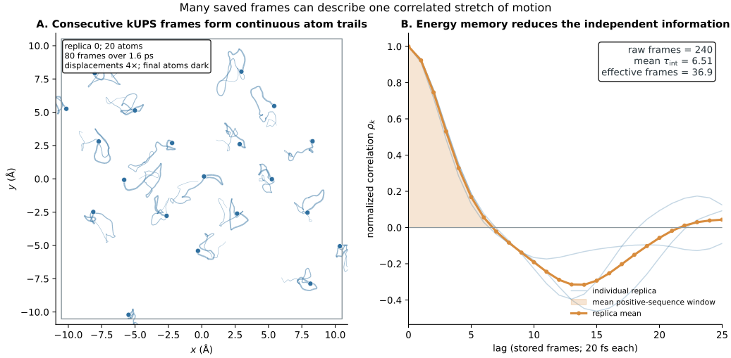
Saving more sparsely would make adjacent stored values less correlated, but it would not create new physics between them. It can reduce storage and analysis cost. For a fixed simulated duration, it usually discards information rather than increasing the total effective information. The cure for inadequate ESS is more independent physical time or better sampling, not a different output stride alone.
Define “long enough” from the claim
No trajectory is long enough for every observable. A mean potential energy may converge before a diffusion coefficient. Local coordination may decorrelate before a phase label. A static average can be useful while a rare transition rate remains completely unsupported.
A practical stopping rule states:
- observable: the exact quantity and estimator being reported;
- warmup: the discarded interval and sensitivity to that choice;
- precision: a target such as \(1.96\operatorname{SE}_{\mathrm{review}}<\epsilon\);
- replicas: agreement of independently initialized runs;
- stability: compatible conclusions after extending every replica.
Block averaging provides a complementary view. As block length exceeds the correlation time, the standard error of block means should approach a plateau. Blocks that are too short retain correlation; blocks that are too long leave too few means for a stable estimate (Flyvbjerg & Petersen, 1989).
Even these gates cannot rescue missing rare events. If replicas never cross the relevant barrier, the measured autocorrelation time describes only motion inside the visited basin. Enhanced sampling or much longer trajectories may be needed; Posts 10 and 11 will address that problem.
Check your understanding
- A trajectory stores 10,000 frames and has \(\tau_{\mathrm{int}}=25\) under this convention. What are \(N_{\mathrm{eff}}\) and the factor multiplying the naive standard error?
- Why can deleting every ninth stored frame reduce the measured lag-one correlation without increasing the information in the simulated path?
- If temperature replicas agree but coordination replicas do not, which observable has failed the convergence check?
- Why can an uncertainty estimate temporarily grow after a trajectory is extended?
For the first question, the answers are 400 effective samples and a fivefold standard-error inflation. The other questions test whether frame storage, observable-specific convergence, and finite-estimator behavior remain distinct.
Simulated time becomes evidence only through an observable
Warmup addresses initialization bias. Autocorrelation measures memory within a retained series. Independent replicas expose between-run disagreement. None can replace the others, and none produces a universal number of MD steps.
A defensible trajectory-length claim names the observable, discard rule, storage interval, integrated-time convention, effective samples, uncertainty, replica spread, and extension test. Post 07 will use that discipline to turn atomic frames into radial, coordination, and dynamical observables.
Reproducibility record and complete trajectory-length dashboard
Run and verify the CPU profile from the locked environment:
git clone https://github.com/sungsoo-ahn/kups-md-tutorials
cd kups-md-tutorials
uv sync --locked

uv run kups-tutorial run 06 --profile smoke
uv run kups-tutorial verify 06 --profile smoke
uv run kups-tutorial verify-notebooks --posts 06 --output-dir notebook-runs
uv run kups-tutorial export-notebook-cells \
  --executed-notebooks-dir notebook-runs \
  --site-root ../sungsoo-ahn.github.io --posts 06 --check
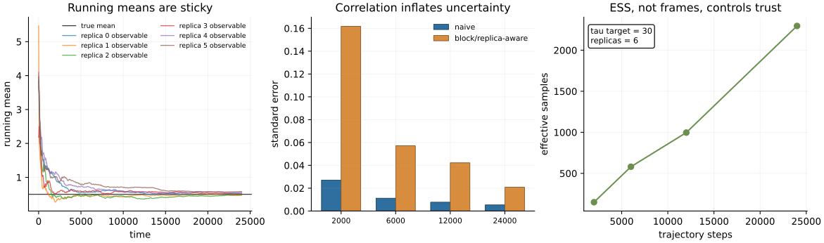
The complete audit dashboard retains the known-mean warmup control, correlation-aware versus naive uncertainty, effective samples across control checkpoints, and both real kUPS observables:
Source and evidence:
References
- Sokal, A. D. (1997). Monte Carlo Methods in Statistical Mechanics: Foundations and New Algorithms. In Functional Integration. ↩
- Chodera, J. D. (2016). A simple method for automated equilibration detection in molecular simulations. Journal of Chemical Theory and Computation, 12, 1799–1805. ↩
- Flyvbjerg, H. & Petersen, H. G. (1989). Error estimates on averages of correlated data. Journal of Chemical Physics, 91, 461–466. ↩