A barostat does not push an instantaneous-pressure display toward a target. It changes the simulation cell. Atomic coordinates must move with that cell, the new density changes forces and virial stress, and the next pressure estimate feeds back into another cell update.
This feedback is noisy by design. Pressure fluctuates strongly in a small atomistic system, and the NPT ensemble also requires volume fluctuations. A flat pressure trace or a rigidly controlled volume can be evidence of the wrong algorithm.
We will expose the isotropic stochastic-cell-rescaling update used by the kUPS csvr_npt path, implement its core in JAX, and then inspect real isotropic and fully flexible kUPS trajectories. The goal is to separate three questions: does the cell respond, has the NPT ensemble equilibrated, and is the force model’s stress physically valid?
- where kinetic and virial terms enter instantaneous pressure;
- why NPT sampling needs volume fluctuations rather than pressure clamping;
- how stochastic cell rescaling updates log volume and affine coordinates;
- how isotropic and flexible-cell barostats represent different degrees of freedom;
- how to distinguish a short response test from an equilibrated NPT result.
Prerequisites: periodic cells and units from Post 01, force-driven integration from Post 02, and thermostat coupling from Post 04.
Pressure is a force response of the whole cell
For a cubic system with pairwise forces, the scalar instantaneous pressure can be written schematically as
\[P_{\mathrm{inst}} = \frac{1}{3V} \left(2K + \sum_{i<j}\mathbf r_{ij}\cdot\mathbf F_{ij}\right).\]The first term is kinetic. The second is the configurational virial: how interatomic forces respond to separation inside the cell. Production codes evaluate a full stress tensor and must handle periodic geometry, many-body potentials, and their own stress sign convention. The scalar pressure is related to the trace of that tensor.
Several consequences follow immediately:
- pressure fluctuates when momenta and configurations fluctuate;
- pressure has much larger frame-to-frame noise than temperature in many small systems;
- changing the volume changes density, pair separations, forces, and the next pressure;
- a learned potential must predict strain derivatives or stress accurately, not only energies at fixed cells.
The barostat consumes this noisy observable. It does not make the observable noise disappear.
The NPT target is a distribution over volume
At target pressure \(P_0\) and temperature \(T\), the isothermal–isobaric ensemble weights a state through the enthalpy-like quantity \(H+P_0V\). In a common shorthand,
\[\pi(\mathbf R,\mathbf P,V) \propto \exp\!\left[-\beta\left(H(\mathbf R,\mathbf P;V)+P_0V\right)\right].\]The exact coordinate measure depends on how positions and the cell are parameterized, but the central point is simple: volume is a sampled variable. At equilibrium its variance is related to the isothermal compressibility,
\[\operatorname{Var}(V) = k_{\mathrm B}T\,\kappa_T\langle V\rangle, \qquad \kappa_T=-\frac{1}{V}\left(\frac{\partial V}{\partial P}\right)_T.\]Suppressing volume fluctuations can therefore corrupt the ensemble even when the average pressure looks plausible (Frenkel & Smit, 2001).
Stochastic cell rescaling is pressure feedback plus noise
The isotropic kUPS path follows stochastic cell rescaling (Bernetti & Bussi, 2020). Define the log-volume increment \(d\epsilon=d\ln V\). A discrete update has the form
\[d\epsilon = \frac{\kappa_T\Delta t}{\tau_P}(P_{\mathrm{inst}}-P_0) + \sqrt{\frac{2k_{\mathrm B}T\kappa_T\Delta t}{\tau_PV}}\,\xi, \qquad \xi\sim\mathcal N(0,1).\]The sign is physically transparent. If internal pressure exceeds the target, the deterministic term is positive and the cell expands. If pressure is too low, it contracts. The random term restores NPT volume fluctuations; deleting it produces a relaxation controller rather than the intended sampler.
Because \(d\epsilon\) changes volume, the linear scale factor in three dimensions is
\[\mu=\exp\!\left(\frac{d\epsilon}{3}\right), \qquad \mathbf h' = \mu\mathbf h, \qquad \mathbf r_i' = \mu\mathbf r_i.\]Scaling both the cell matrix \(\mathbf h\) and all positions preserves fractional coordinates. Scaling only one would instantaneously change where atoms sit relative to the periodic box. kUPS also clamps \(\mu\) to a safe per-step range; a repeatedly active clamp indicates that the timestep, coupling, pressure, or initial state needs review.
Put the kUPS cell update into JAX
The collapsed setup selects a CPU backend and imports the configuration and real kUPS runner.
Python
from pathlib import Path
import csv
import os

os.environ.setdefault("JAX_PLATFORMS", "cpu")
import jax
from jax import Array
import jax.numpy as jnp

from IPython.display import Image, display

from kups_md_tutorials.config import load_barostat_spec
from kups_md_tutorials.jax_reference import (
    BOLTZMANN_EV_PER_K,
    IsotropicCellState,
)
from kups_md_tutorials.barostat_visuals import generate_post05_cell_response_visual
from kups_md_tutorials.kups_engine import (
    load_kups_md_experiment,
    run_kups_md_experiment,
    write_kups_thermodynamic_samples,
)

repo_root = Path.cwd()
if not (repo_root / "configs").exists():
    repo_root = repo_root.parent
os.chdir(repo_root)
The open cell below mirrors the core operations of kUPS stochastic cell rescaling without its table/lens abstractions. A linear pressure–volume law provides a known equilibrium. The JAX state contains both positions and the cell, and a single random key controls each log-volume update.
Python
def stochastic_cell_rescaling_step(
    state: IsotropicCellState,
    current_pressure: Array,
    key: Array,
    *,
    time_step: float,
    target_pressure: float,
    pressure_coupling_time: float,
    compressibility: float,
    temperature: float,
    minimum_scale_factor: float = 0.995,
    boltzmann_constant: float = BOLTZMANN_EV_PER_K,
) -> tuple[IsotropicCellState, Array]:
    """Apply the isotropic stochastic cell-rescaling core used by kUPS."""

    volume = jnp.abs(jnp.linalg.det(state.cell))
    pressure_feedback = (
        (time_step / pressure_coupling_time)
        * compressibility
        * (current_pressure - target_pressure)
    )
    random_log_volume = jnp.sqrt(
        2.0
        * boltzmann_constant
        * temperature
        * compressibility
        * time_step
        / (pressure_coupling_time * volume)
    ) * jax.random.normal(key, dtype=state.positions.dtype)
    log_volume_change = pressure_feedback + random_log_volume

    length_scale = jnp.exp(log_volume_change / 3.0)
    length_scale = jnp.clip(
        length_scale,
        minimum_scale_factor,
        1.0 / minimum_scale_factor,
    )
    next_state = IsotropicCellState(
        positions=state.positions * length_scale,
        cell=state.cell * length_scale,
    )
    return next_state, length_scale


spec = load_barostat_spec("05", "full")
experiment = spec.experiment
reference_volume = experiment.equilibrium_volume
initial_length = (0.9 * reference_volume) ** (1.0 / 3.0)
initial = IsotropicCellState(
    positions=initial_length * jnp.array([[0.25, 0.25, 0.25], [0.75, 0.75, 0.75]]),
    cell=initial_length * jnp.eye(3),
)


def pressure_from_volume(volume):
    return experiment.target_pressure - (volume - reference_volume) / (
        experiment.compressibility * reference_volume
    )


for index, case in enumerate(experiment.barostats):
    keys = jax.random.split(
        jax.random.fold_in(jax.random.PRNGKey(experiment.seed), index),
        experiment.num_steps,
    )

    def advance(state, step_key):
        volume = jnp.abs(jnp.linalg.det(state.cell))
        pressure = pressure_from_volume(volume)
        next_state, length_scale = stochastic_cell_rescaling_step(
            state,
            pressure,
            step_key,
            time_step=experiment.time_step,
            target_pressure=experiment.target_pressure,
            pressure_coupling_time=case.relaxation_time,
            compressibility=experiment.compressibility,
            temperature=experiment.temperature,
            minimum_scale_factor=0.9,
            boltzmann_constant=1.0,
        )
        return next_state, (volume, pressure, length_scale)

    _, (volumes, pressures, scales) = jax.lax.scan(advance, initial, keys)
    sampled = volumes[experiment.warmup_steps::experiment.sample_every]
    expected_variance = (
        experiment.temperature * experiment.compressibility * reference_volume
    )
    print(
        f"tau_P={case.relaxation_time:g}: mean V={jnp.mean(sampled):.2f}, "
        f"Var(V)/target={jnp.var(sampled, ddof=1) / expected_variance:.3f}, "
        f"mean P={jnp.mean(pressures[experiment.warmup_steps:]):.3f}"
)tau_P=0.5: mean V=1000.04, Var(V)/target=1.054, mean P=1.001
tau_P=2: mean V=999.99, Var(V)/target=1.086, mean P=1.001
tau_P=8: mean V=999.48, Var(V)/target=0.957, mean P=1.051
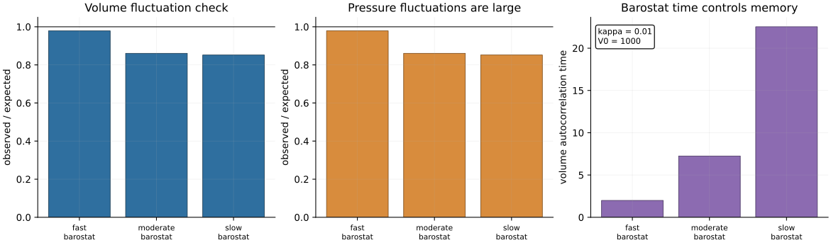
All three coupling times recover a mean volume near 1,000 and a variance close to the analytic target of 10. Their variance ratios are 1.054, 1.086, and 0.957. The slowest run has a mean pressure of 1.051 rather than 1.000 even after the same number of steps because its cell retains more memory.
The longer committed control quantifies that memory. Increasing \(\tau_P\) from 0.5 to 8 raises the volume integrated autocorrelation time from 1.99 to 22.53 saved samples. Effective volume samples fall from about 1,256 to
- A smooth slow response is not the same as efficient sampling.
kUPS exposes scalar and tensor cell dynamics
The two production paths in this lesson do not represent the same cell:
| kUPS integrator | Cell degrees of freedom | Per-step structure |
|---|---|---|
csvr_npt | one isotropic volume mode | CSVR thermostat → velocity Verlet → stochastic cell rescaling → new forces/stress |
baoab_npt_langevin | lower-triangular flexible cell and cell momentum | coupled atom/cell kicks, drifts, and Langevin refreshes in a BAOAB palindrome |
Isotropic rescaling can change density but not angles or relative edge ratios. The flexible formulation introduces a cell-momentum tensor and can respond to anisotropic stress and shear. kUPS implements the Gao–Fang–Wang extended-cell Langevin scheme for that path (Gao et al., 2016).
More degrees of freedom are not automatically better. Liquids often need only isotropic pressure control. Crystals may require anisotropic relaxation, but a flexible cell also exposes shear instabilities and weaknesses in a potential’s stress predictions.
Pressure units must cross the API boundary correctly
kUPS stores virial stress in its internal \(\mathrm{eV}/\mathring{A}^3\) units. The analysis layer converts before naming a value pressure_pa:
A unit test injects a one-pascal diagonal stress and requires a one-pascal pressure result. Without that boundary test, a plausible-looking trace could be wrong by eleven orders of magnitude.
Run both moving-cell paths through kUPS
The next cell runs 32-atom CPU smoke cases through kups.application.simulations.md.run, writes separate HDF5 files, and derives volume and pressure traces from those files.
Python
kups_spec = load_kups_md_experiment("05", "smoke")
raw_dir = Path("notebook-runs/post-05-raw")
kups_result = run_kups_md_experiment(kups_spec, raw_run_dir=raw_dir, quiet=True)
trace_path = Path("notebook-runs/post-05-kups-npt.csv")
write_kups_thermodynamic_samples(trace_path, kups_spec, raw_run_dir=raw_dir)
rows = list(csv.DictReader(trace_path.open()))

evidence = []
for case in kups_result.cases:
    case_rows = [row for row in rows if row["case"] == case.name]
    ratios = [float(row["volume_ratio"]) for row in case_rows]
    pressures = [float(row["pressure_pa"]) / 1e6 for row in case_rows]
    evidence.append(
        {
            "case": case.name,
            "integrator": case.integrator,
            "frames": case.frame_count,
            "final V / V_first": round(ratios[-1], 4),
            "stored volume span": round(max(ratios) - min(ratios), 4),
            "final pressure (MPa)": round(pressures[-1], 1),
            "devices": case.observed_devices,
        }
    )
evidence[{'case': 'isotropic_tau_500fs',
'integrator': 'csvr_npt',
'frames': 16,
'final V / V_first': 1.0783,
'stored volume span': 0.0783,
'final pressure (MPa)': 142.7,
'devices': ('cpu:cpu',)},
{'case': 'flexible_tau_1000fs',
'integrator': 'baoab_npt_langevin',
'frames': 16,
'final V / V_first': 1.0573,
'stored volume span': 0.0651,
'final pressure (MPa)': 109.2,
'devices': ('cpu:cpu',)}]The 16-frame smoke runs establish execution, not equilibration. The isotropic cell grows by 7.83% relative to its first stored volume and ends at 142.7 MPa; the flexible case grows by 5.73% and ends at 109.2 MPa. Both are still in a large transient.
The full profile uses 256 atoms, 200 warmup steps, 800 production steps, and 80 stored frames over 1.6 ps. All three workers observed an NVIDIA RTX A5000:
| Full kUPS case | Mean \(T\) | Mean \(P\) | Final \(V/V_{\mathrm{first}}\) | Final \(P\) |
|---|---|---|---|---|
| CSVR–NPT, \(\tau_P=0.5\) ps | 95.0 K | 38.2 MPa | 1.0970 | 30.8 MPa |
| CSVR–NPT, \(\tau_P=2.0\) ps | 100.6 K | 139.0 MPa | 1.0915 | 61.6 MPa |
| flexible BAOAB–NPT, \(\tau_P=1.0\) ps | 99.1 K | 3.1 MPa | 1.0921 | 7.6 MPa |
The target is 10 MPa. These means do not rank integrators because the stored window begins during response from a dense high-pressure cell. The slow isotropic run retains more of that initial condition. The flexible case crosses the target, but one crossing and a nearby final frame do not establish equilibrium.
Temperature and pressure must also be read separately. The slow isotropic case has a reasonable mean temperature while its pressure remains far from the target. Thermostat equilibration does not imply barostat equilibration.
Watch the periodic cell expand around real atoms
The next figure puts the feedback equation above actual positions from the full fast-isotropic HDF5 trajectory. The same physical scale is used in both atom panels, so the cell-edge change is not a drawing trick.
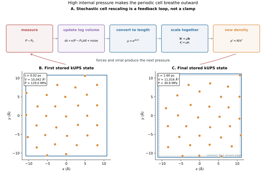
The cubic edge grows only about 3.1% because volume scales as length cubed. The atomic layer becomes less dense, which weakens the high internal pressure. The final 30.8 MPa remains above target: feedback is working, but the bounded run has not finished relaxing.
The flexible-cell HDF5 evidence surface records volume but not the full cell matrix at every stored step. This article therefore makes no visual or quantitative claim about cell angles, shear, or shape distributions for that case.
A successful NPT study needs four gates
- Execution: every intended NPT path compiles, writes finite cells and stress, and records its actual device.
- Response: starting from controlled compressed and expanded cells, volume moves in the physically expected direction while temperature remains plausible.
- Sampling: longer independent replicas give stable volume/pressure statistics with autocorrelation-aware uncertainty and warmup sensitivity.
- Model validity: reference calculations support energies, forces, and stress over the strained configurations visited by the cell.
This chapter completes the first two for a bounded Lennard-Jones implementation test. Eighty frames cannot establish compressibility, an argon equation of state, or a production NPT uncertainty.
For a crystal, the third gate also needs stored cell vectors, shape and angle distributions, and anisotropic stress. For an MLIP, the fourth gate is often the hardest: an NPT run can be numerically stable while the model extrapolates under strain.
Check your understanding
- If \(P_{\mathrm{inst}}>P_0\), what is the sign of the deterministic \(d\epsilon\) term, and why does that reduce pressure in a compressed cell?
- Why must atomic positions and the cell matrix use the same linear scale \(\mu\)?
- What ensemble error appears if the stochastic term is deleted but the mean pressure still reaches the target?
- Which stored data are missing if you want to validate a flexible-cell shear claim?
The third question distinguishes relaxation from sampling. Reaching a target mean is not enough when the target ensemble specifies fluctuations.
A barostat controls a distribution by changing geometry
Pressure is not an independent knob. It is computed from kinetic motion, forces, and cell geometry. A barostat changes geometry, the potential responds, and the feedback repeats. Stochastic cell rescaling makes that loop explicit; the flexible-cell method generalizes it to tensor degrees of freedom.
A defensible NPT result reports the cell model, pressure and temperature couplings, compressibility, timestep, warmup, cell response, volume and stress fluctuations, effective samples, replicas, stored cell surface, and validation domain of the potential. Post 06 will ask how long such a correlated trajectory must run before its averages become informative.
Reproducibility record and complete NPT dashboard
Run and verify the CPU profile from the locked environment:
git clone https://github.com/sungsoo-ahn/kups-md-tutorials
cd kups-md-tutorials
uv sync --locked

uv run kups-tutorial run 05 --profile smoke
uv run kups-tutorial verify 05 --profile smoke
uv run kups-tutorial verify-notebooks --posts 05 --output-dir notebook-runs
uv run kups-tutorial export-notebook-cells \
  --executed-notebooks-dir notebook-runs \
  --site-root ../sungsoo-ahn.github.io --posts 05 --check
The full audit dashboard retains volume, pressure, temperature, and response-versus-fluctuation traces for all three full kUPS cases:
Source and evidence:
References
- Frenkel, D. & Smit, B. (2001). Understanding Molecular Simulation: From Algorithms to Applications. Academic Press. ↩
- Bernetti, M. & Bussi, G. (2020). Pressure control using stochastic cell rescaling. Journal of Chemical Physics, 153, 114107. ↩
- Gao, X., Fang, J. & Wang, H. (2016). Sampling the isothermal–isobaric ensemble by Langevin dynamics. Journal of Chemical Physics, 144, 124113. ↩