A thermostat is not a correction that pushes a temperature display toward a number. It changes momenta throughout the trajectory. With the right balance of friction and noise, that altered dynamics samples the canonical ensemble. With a different coupling strength or algorithm, it can sample similar static distributions while producing different time correlations.
That distinction decides whether a trajectory can support a claim. Mean energy, structure, and other equilibrium averages need the right ensemble. Diffusion, spectra, and rate estimates also depend on how motion unfolds in time. We will make both requirements visible: first in a transparent JAX implementation of BAOAB Langevin dynamics, then in real BAOAB and CSVR kUPS runs.
- why temperature is a fluctuating kinetic-energy estimator, not a controlled state variable at every step;
- how friction and random force combine through fluctuation–dissipation;
- what the five letters in BAOAB do to positions and momenta;
- how BAOAB and CSVR can share an ensemble target but alter dynamics differently;
- which evidence is needed before using a thermostatted trajectory for a static or dynamical observable.
Prerequisites: the state and temperature estimator from Post 01, the integrator map from Post 02, and the error distinctions from Post 03.
NVE and NVT answer different physical questions
For positions \(\mathbf R\), momenta \(\mathbf P\), and Hamiltonian
\[H(\mathbf R,\mathbf P) = U(\mathbf R) + \sum_i \frac{\lVert\mathbf p_i\rVert^2}{2m_i},\]an ideal microcanonical trajectory keeps \(H\) fixed. It represents an isolated system with fixed particle number, volume, and energy: the NVE ensemble.
A system in thermal contact with a much larger heat bath can exchange energy. At temperature \(T\), its canonical density is
\[\pi(\mathbf R,\mathbf P) = \frac{1}{Z} \exp\!\left[-\beta H(\mathbf R,\mathbf P)\right], \qquad \beta=\frac{1}{k_{\mathrm B}T}.\]This is the NVT ensemble. A thermostat modifies the equations of motion so that this density is stationary. It should not conserve the system’s ordinary total energy: energy must enter and leave through the modelled bath.
The practical question is therefore not “does energy drift under NVT?” It is “does the stationary trajectory represent the intended canonical density, and what dynamical information survives the coupling?”
Temperature is a noisy observable
Classical MD infers an instantaneous kinetic temperature from
\[K=\sum_i\frac{\lVert\mathbf p_i\rVert^2}{2m_i}, \qquad T_{\mathrm{inst}}=\frac{2K}{f k_{\mathrm B}},\]where \(f\) is the number of active degrees of freedom. If center-of-mass translation was removed, three degrees are usually subtracted. Constraints remove more.
Even a perfect canonical sampler does not make \(T_{\mathrm{inst}}=T\) in every frame. In the canonical ensemble,
\[\frac{2K}{k_{\mathrm B}T}\sim\chi_f^2, \qquad \langle K\rangle=\frac{f}{2}k_{\mathrm B}T.\]The fluctuations are part of the ensemble. A controller that clamps kinetic energy exactly can suppress the distribution it is meant to sample. We care about the distribution and its correlations, not whether a temperature curve looks smooth.
Langevin dynamics balances forgetting and noise
In momentum form, Langevin dynamics is
\[d\mathbf R_i=\frac{\mathbf p_i}{m_i}\,dt,\] \[d\mathbf p_i = \mathbf F_i(\mathbf R)\,dt - \gamma\mathbf p_i\,dt + \sqrt{2\gamma m_i k_{\mathrm B}T}\,d\mathbf W_i.\]The friction \(-\gamma\mathbf p_i\) erases momentum memory. The Wiener increment \(d\mathbf W_i\) adds random momentum. Their amplitudes cannot be chosen independently: fluctuation–dissipation is what leaves the Maxwell momentum distribution stationary.
The timescale \(\gamma^{-1}\) gives useful intuition. Weak friction allows long ballistic or oscillatory memory. Strong friction rapidly randomizes momenta, but positions can then diffuse slowly through an overdamped landscape. Stronger coupling is not automatically faster sampling.
BAOAB makes the heat exchange explicit
BAOAB splits one timestep into five exactly named operations (Leimkuhler & Matthews, 2013). Let \(c=\exp(-\gamma\Delta t)\) and draw a fresh standard normal vector \(\boldsymbol\xi_n\):
\[\begin{aligned} \mathbf p^{(1)} &= \mathbf p_n + \frac{\Delta t}{2}\mathbf F(\mathbf R_n), &&\text{B: force kick},\\ \mathbf R^{(1)} &= \mathbf R_n + \frac{\Delta t}{2}\frac{\mathbf p^{(1)}}{\mathbf m}, &&\text{A: half drift},\\ \mathbf p^{(2)} &= c\mathbf p^{(1)} + \sqrt{\mathbf m k_{\mathrm B}T(1-c^2)}\,\boldsymbol\xi_n, &&\text{O: heat bath},\\ \mathbf R_{n+1} &= \mathbf R^{(1)} + \frac{\Delta t}{2}\frac{\mathbf p^{(2)}}{\mathbf m}, &&\text{A: half drift},\\ \mathbf p_{n+1} &= \mathbf p^{(2)} + \frac{\Delta t}{2}\mathbf F(\mathbf R_{n+1}), &&\text{B: force kick}. \end{aligned}\]Only the O step exchanges heat. Its variance explains the noise amplitude. If \(\operatorname{Var}(\mathbf p)=\mathbf m k_{\mathrm B}T\) before the step, then
\[\operatorname{Var}(c\mathbf p+\sigma\boldsymbol\xi) =c^2\mathbf m k_{\mathrm B}T +\mathbf m k_{\mathrm B}T(1-c^2) =\mathbf m k_{\mathrm B}T.\]The deterministic B and A operations are the same force and drift ideas used by velocity Verlet. The O operation is the new physics.
Write those five operations in JAX
The collapsed setup chooses the CPU backend, enables float64 for the analytic control, and imports the real kUPS workflow.
Python
import jax
jax.config.update("jax_enable_x64", True)
from jax import Array
import jax.numpy as jnp

from kups_md_tutorials.config import load_thermostat_spec
from kups_md_tutorials.kups_engine import (
    load_kups_md_experiment,
    load_kups_result,
    run_kups_md_experiment,
)
from kups_md_tutorials.jax_reference import (
    EnergyFunction,
    ParticleState,
)
from kups_md_tutorials.thermostat_visuals import (
    generate_post04_thermostat_mechanism,
)
The open cell below is the algorithm rather than a wrapper around it. The PRNG key is explicit, jax.random.split supplies one independent key per step, and jax.lax.scan carries the immutable state. Forces still come from -jax.grad(energy_fn).
Python
def baoab_langevin_step(
    energy_fn: EnergyFunction,
    state: ParticleState,
    key: Array,
    *,
    time_step: float,
    friction: float,
    temperature: float,
    boltzmann_constant: float = 1.0,
) -> ParticleState:
    """Apply one B-A-O-A-B Langevin step to positions and momenta."""

    forces = -jax.grad(energy_fn)(state.positions)
    momenta = state.momenta + 0.5 * time_step * forces  # B: kick
    positions = state.positions + 0.5 * time_step * (
        momenta / state.masses[:, None]
    )  # A: drift

    memory = jnp.exp(-friction * time_step)
    noise_scale = jnp.sqrt(
        state.masses[:, None]
        * boltzmann_constant
        * temperature
        * (1.0 - memory**2)
    )
    noise = jax.random.normal(key, state.momenta.shape, dtype=state.momenta.dtype)
    momenta = memory * momenta + noise_scale * noise  # O: heat bath

    positions = positions + 0.5 * time_step * (
        momenta / state.masses[:, None]
    )  # A: drift
    forces = -jax.grad(energy_fn)(positions)
    momenta = momenta + 0.5 * time_step * forces  # B: kick
    return ParticleState(positions, momenta, state.masses)


def simulate_baoab_langevin(
    energy_fn: EnergyFunction,
    initial_state: ParticleState,
    key: Array,
    *,
    time_step: float,
    friction: float,
    temperature: float,
    num_steps: int,
    boltzmann_constant: float = 1.0,
) -> tuple[ParticleState, ParticleState]:
    """Scan BAOAB with one independent random key per thermostat step."""

    keys = jax.random.split(key, num_steps)

    def advance(
        state: ParticleState,
        step_key: Array,
    ) -> tuple[ParticleState, ParticleState]:
        next_state = baoab_langevin_step(
            energy_fn,
            state,
            step_key,
            time_step=time_step,
            friction=friction,
            temperature=temperature,
            boltzmann_constant=boltzmann_constant,
        )
        return next_state, next_state

    return jax.lax.scan(advance, initial_state, keys)


def oscillator_energy(positions):
    return 0.5 * jnp.sum(positions**2)


initial = ParticleState(jnp.array([[1.0]]), jnp.array([[0.0]]), jnp.array([1.0]))
for index, case in enumerate(full_spec.experiment.thermostats):
    _, trajectory = simulate_baoab_langevin(
        oscillator_energy,
        initial,
        jax.random.fold_in(jax.random.PRNGKey(full_spec.experiment.seed), index),
        time_step=full_spec.experiment.time_step,
        friction=case.gamma,
        temperature=full_spec.experiment.temperature,
        num_steps=full_spec.experiment.num_steps,
    )
    q = trajectory.positions[full_spec.experiment.warmup_steps::10, 0, 0]
    p = trajectory.momenta[full_spec.experiment.warmup_steps::10, 0, 0]
    print(
        f"gamma={case.gamma:g}: Var(q)={jnp.var(q):.3f}, "
        f"Var(p)={jnp.var(p):.3f}, <K>={jnp.mean(0.5 * p**2):.3f}"
)gamma=0.1: Var(q)=1.102, Var(p)=1.091, <K>=0.546
gamma=1: Var(q)=0.997, Var(p)=1.000, <K>=0.500
gamma=5: Var(q)=0.862, Var(p)=0.970, <K>=0.485
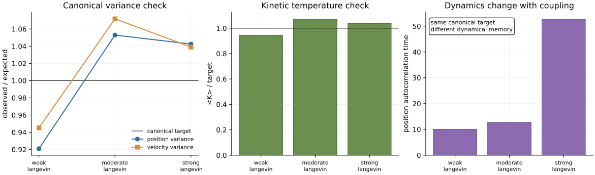
For the unit harmonic oscillator, the exact canonical targets are \(\operatorname{Var}(q)=\operatorname{Var}(p)=1\) and \(\langle K\rangle=1/2\). The moderate-coupling run reports 0.997, 1.000, and 0.500. The weak and strong runs deviate more in this finite record: their position variances are 1.102 and 0.862.
Those deviations do not by themselves rank the thermostats. The saved points are correlated, so 3,500 stored values are fewer than 3,500 independent draws. In the longer committed control, the position effective sample count is about 348 for weak coupling but only 66 for strong coupling. Uncertainty must use effective samples, not the raw frame count.
BAOAB and CSVR do not modify momentum the same way
BAOAB applies an independent Ornstein–Uhlenbeck refresh to each momentum component. Canonical stochastic velocity rescaling (CSVR) instead evolves the total kinetic energy with a stochastic process and applies one shared scale factor,
\[\mathbf p_i' = \alpha\mathbf p_i,\]to all momenta. The random construction of \(\alpha\) preserves the canonical kinetic-energy distribution rather than forcing one deterministic kinetic energy (Bussi et al., 2007).
| Property | BAOAB Langevin | CSVR |
|---|---|---|
| Bath action | component-wise friction and noise | one stochastic global rescaling |
| Main coupling parameter | friction \(\gamma\) | relaxation time \(\tau_T\) |
| Canonical target | positions and momenta | kinetic energy, coupled to MD positions |
| Dynamical effect | local momentum decorrelation | global kinetic-mode coupling |
| Same trajectories expected? | no | no |
Both can be valid canonical samplers. Neither gives thermostat-independent real-time dynamics merely because the mean temperature is correct.
Run both thermostats through kUPS
The next cell performs two new 32-atom CPU runs through kups.application.simulations.md.run. It reopens each HDF5 file and prints the integrator, frame and atom counts, block temperature estimate, observed device, and content hash. It also prints the committed full-profile record.
Python
kups_spec = load_kups_md_experiment("04", "smoke")
kups_result = run_kups_md_experiment(
    kups_spec,
    raw_run_dir=Path("runs/notebook-post-04/smoke"),
    quiet=True,
)

for case in kups_result.cases:
    print(
        case.name,
        f"integrator={case.integrator}",
        f"frames={case.frame_count}",
        f"atoms={case.atom_count}",
        f"T={case.temperature_k['mean']:.2f} +/- {case.temperature_k['sem']:.2f} K",
        f"device={','.join(case.observed_devices)}",
        f"hdf5={case.hdf5_sha256[:12]}",
    )

production = load_kups_result(Path("results/post-04/full/kups_md_summary.json"))
for case in production.cases:
    print(
        f"production {case.name}",
        f"frames={case.frame_count}",
        f"atoms={case.atom_count}",
        f"T={case.temperature_k['mean']:.2f} +/- {case.temperature_k['sem']:.2f} K",
        f"device={case.observed_devices[0]}",
        f"hdf5={case.hdf5_sha256[:12]}",
    )
baoab_nvt integrator=baoab_langevin frames=8 atoms=32 T=92.55 +/- 1.84 K device=cpu:cpu hdf5=59076b2f3f61
csvr_nvt integrator=csvr frames=8 atoms=32 T=94.06 +/- 5.30 K device=cpu:cpu hdf5=245e6765e27c
production baoab_nvt frames=1000 atoms=256 T=99.97 +/- 0.28 K device=gpu:NVIDIA RTX A5000 hdf5=79f8fe809975
production csvr_nvt frames=1000 atoms=256 T=99.85 +/- 0.42 K device=gpu:NVIDIA RTX A5000 hdf5=2d63432d3018
The smoke cases produce only eight stored frames. Their 92.55 K BAOAB and 94.06 K CSVR estimates confirm executable, finite HDF5 analysis; they are not convergence evidence for a 100 K target.
The quantitative evidence comes from 256 atoms, 20,000 warmup steps, 20,000 production steps, and 1,000 stored frames per thermostat:
| Full kUPS case | Coupling | Mean temperature | Stored frames | Observed device |
|---|---|---|---|---|
| BAOAB Langevin | \(\gamma=0.01\ \mathrm{fs}^{-1}\) | 99.970 ± 0.279 K | 1,000 | NVIDIA RTX A5000 |
| CSVR | \(\tau_T=100\ \mathrm{fs}\) | 99.851 ± 0.424 K | 1,000 | NVIDIA RTX A5000 |
The ± values are block standard errors of the mean, not the width of instantaneous temperature fluctuations. Both means support a narrow claim: under these protocols, the low-order kinetic-temperature estimate is consistent with 100 K. They do not establish identical configurational sampling, efficiency, or dynamics.
See where the bath enters an atomic trajectory
The top row of the next figure turns the equations into a state transition: B changes momentum through force, A moves the atom, and O replaces part of the old momentum with a thermal draw. The lower panels use actual atom positions from the two full kUPS HDF5 files.
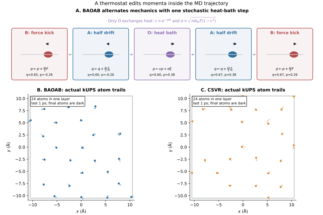
The trails are short because a solid-like argon atom moves around its local environment over this window. A thermostat changes those motions through momenta, but an endpoint picture cannot validate an ensemble. Distributional and correlation diagnostics remain necessary.
Correlation determines how much information was collected
For a sampled observable \(A_n\) with normalized autocorrelation \(\rho(k)\), a common integrated autocorrelation estimate is
\[\tau_{\mathrm{int}} =1+2\sum_{k=1}^{k_{\max}}\rho(k), \qquad N_{\mathrm{eff}}\approx\frac{N}{\tau_{\mathrm{int}}}.\]In the committed oscillator control, increasing \(\gamma\) from 0.1 to 5.0 reduces one-step velocity correlation from 0.958 to 0.355. Yet the position autocorrelation time grows from 10.1 to 52.7 saved samples. Momentum forgets quickly while the coordinate explores slowly: the overdamped regime.
This is why a thermostat should be tuned against the observable of interest. Temperature relaxation alone cannot reveal sampling efficiency.
Choose a production protocol from the claim
For equilibrium averages, a validated NVT production run can be appropriate. Check kinetic moments, configurational observables, equilibration, correlation times, and independent replicas.
For diffusion coefficients, velocity autocorrelation functions, vibrational spectra, or rates, thermostat perturbations can enter the answer directly. A common design is:
- equilibrate positions and momenta under NVT;
- transfer that exact final state into NVE;
- verify NVE energy behavior;
- compute the dynamical observable over multiple independent segments.
The current real kUPS evidence in this chapter validates separate NVT runs; it does not demonstrate an exact kUPS NVT-to-NVE state handoff. A reduced-unit control exists in the audit artifacts, but it is not a substitute for that production operation.
The same caution applies to machine-learned potentials. A strong thermostat can continually remove energy injected by noisy or extrapolative forces. A stable temperature is therefore not evidence that the force model is valid.
Check your understanding
- If \(\gamma\) doubles, which BAOAB line changes directly? Which two terms must change together to preserve the same momentum variance?
- Why is a perfectly flat instantaneous-temperature trace suspicious in an NVT simulation?
- Two thermostats give the same mean temperature. What additional checks are needed before comparing a diffusion coefficient?
- Why can 3,500 stored oscillator states contain only about 66 effective position samples?
The first question is the algorithmic core: friction without matching noise cools the system, while noise without matching friction heats it.
A thermostat defines sampling dynamics, not just temperature
BAOAB makes the intervention easy to locate. Four substeps follow mechanics; one substep exchanges momentum with a bath. CSVR performs a different stochastic intervention through global kinetic energy. Both choices can reach the canonical target, but they need not preserve the same temporal path.
A defensible thermostat claim therefore names the ensemble, algorithm, coupling time, equilibration period, sampled observable, correlation analysis, and hardware-backed execution evidence. Post 05 will add a second bath variable—the simulation cell—and ask the same questions about pressure.
Reproducibility record and complete diagnostic dashboard
Run and verify the CPU profile from the locked environment:
git clone https://github.com/sungsoo-ahn/kups-md-tutorials
cd kups-md-tutorials
uv sync --locked

uv run kups-tutorial run 04 --profile smoke
uv run kups-tutorial verify 04 --profile smoke
uv run kups-tutorial verify-notebooks --posts 04 --output-dir notebook-runs
uv run kups-tutorial export-notebook-cells \
  --executed-notebooks-dir notebook-runs \
  --site-root ../sungsoo-ahn.github.io --posts 04 --check
The full audit dashboard retains the canonical variance, kinetic moment, position-memory, and real kUPS temperature panels:
Source and evidence:
References
- Leimkuhler, B. & Matthews, C. (2013). Rational construction of stochastic numerical methods for molecular sampling. Applied Mathematics Research eXpress, 2013(1), 34–56. ↩
- Bussi, G., Donadio, D. & Parrinello, M. (2007). Canonical sampling through velocity rescaling. Journal of Chemical Physics, 126, 014101. ↩