An energy trace is evidence, not a verdict. A wider trace can come from a large timestep, accumulated arithmetic error, or forces that do not match the reported energy. A flat trace can belong to the wrong conservative potential. One number called “energy drift” cannot distinguish those mechanisms.
We will separate them on a harmonic oscillator whose exact trajectory is known. Then we will compare matched kUPS trajectories atom by atom. The goal is to replace the question “is the simulation accurate?” with smaller questions that an experiment can answer.
- how timestep, arithmetic, initial-state, and force-model errors differ;
- why velocity Verlet can have bounded energy error but growing phase error;
- how to expose the force function and arithmetic policy in JAX;
- why conserving energy does not validate a potential;
- how matched seeds and atom-level displacement reveal trajectory divergence.
Prerequisites: the initialized state from Post 01 and the velocity-Verlet map from Post 02.
“Trajectory error” is not one object
Let \(z(t)=(\mathbf{R}(t),\mathbf{P}(t))\) be the exact trajectory under a chosen potential \(U\). A program produces discrete states
\[z_{n+1}=\Phi_{\Delta t,p,\widetilde U}(z_n).\]Here \(\Phi\) is the implemented update, \(\Delta t\) is the timestep, \(p\) denotes the arithmetic policy, and \(\widetilde U\) is the energy model used by the program. Each subscript creates a different comparison:
- Timestep error: compare the discrete map with continuous dynamics under the same \(U\).
- Arithmetic error: compare implementations of the same discrete map under different dtypes or rounding policies.
- Force-model error: compare trajectories under \(\widetilde U\) and the scientifically intended \(U\).
- Initial-state variation: compare independent draws from the same stated initialization distribution.
The first three change the computed dynamics. The fourth does not indicate a fault; it measures how much the protocol depends on one sampled state.
We also need to choose what is compared. Position error, energy error, a radial distribution, and a diffusion coefficient can rank two methods differently. Accuracy only has meaning relative to an observable and a time window.
Timestep error changes the discrete flow
Velocity Verlet approximates a continuous path with finite kick–drift–kick updates. For a smooth system, reducing \(\Delta t\) usually reduces local truncation error. After many steps, the numerical trajectory can still move out of phase with the exact one.
The unit harmonic oscillator makes that phase error visible:
\[\ddot q=-q, \qquad q(t)=\cos t, \qquad E(q,p)=\frac{q^2+p^2}{2},\]for \(q(0)=1\) and \(p(0)=0\). The exact energy is \(1/2\) at every time. A symplectic method such as velocity Verlet usually oscillates around that value instead of producing monotonic loss or gain. It follows the flow of a nearby modified Hamiltonian (Hairer et al., 2006).
Bounded energy therefore does not imply a small position error at late times. The numerical oscillator can have the right amplitude and the wrong phase.
Arithmetic error perturbs every update
Floating-point numbers keep a finite number of significant bits. Each force, sum, and state update is rounded to a representable value. The effect depends on dtype, hardware, operation order, system size, and the number of steps (Higham, 2002).
Roundoff is not equivalent to a larger timestep:
- timestep error changes the mathematical map before arithmetic is applied;
- roundoff perturbs the evaluation of that chosen map;
- reducing \(\Delta t\) increases the number of updates needed for a fixed physical duration, so smaller steps do not monotonically remove roundoff.
JAX defaults and accelerator support matter here. Enabling float64 in Python does not guarantee that every deployed kernel has the same throughput or reduction order. Precision is part of the execution contract, not a cosmetic array property.
Force error can be conservative or inconsistent
Suppose the intended energy is \(U\) but the program uses \(\widetilde U=0.98U\). If forces are computed consistently,
\[\widetilde{\mathbf F}(\mathbf R) =-\nabla_{\mathbf R}\widetilde U(\mathbf R),\]the simulation can conserve \(\widetilde U+K\) extremely well. It still follows the wrong Hamiltonian for a claim about \(U\).
A different failure occurs when the code reports \(U\) but propagates with a force that is not \(-\nabla U\). Energy exchange between potential and kinetic terms is then inconsistent. An NVE trace can expose that mismatch, but it cannot prove that a consistently differentiated model is physically accurate.
This distinction is central for machine-learned interatomic potentials. Force consistency is a software and differentiation property. Agreement with reference quantum mechanics is a model-validation property.
Put the error sources into JAX
The setup chooses a CPU backend, enables float64 for the analytic control, and imports the real kUPS workflow. It begins collapsed.
Python
from pathlib import Path
import os

repo_root = Path.cwd()
if not (repo_root / "configs").exists():
    repo_root = repo_root.parent
os.chdir(repo_root)
os.environ.setdefault("JAX_PLATFORMS", "cpu")

from collections.abc import Callable
import jax
jax.config.update("jax_enable_x64", True)
from jax import Array
import jax.numpy as jnp
from IPython.display import Image, display
from kups_md_tutorials.config import load_error_spec
from kups_md_tutorials.jax_reference import ParticleState, kinetic_energy
from kups_md_tutorials.kups_engine import (
    load_kups_md_experiment,
    run_kups_md_experiment,
)
The open cell makes the force function an explicit input to Verlet. An optional quantizer rounds positions and momenta after every step. This quantizer is deliberately crude; it creates an arithmetic floor large enough to inspect in a short example.
Python
type ForceFunction = Callable[[Array], Array]


def velocity_verlet_step_from_force(
    force_fn: ForceFunction,
    state: ParticleState,
    time_step: float,
) -> ParticleState:
    """Advance Verlet while exposing the force model as an explicit input."""

    forces = force_fn(state.positions)
    half_momenta = state.momenta + 0.5 * time_step * forces
    positions = state.positions + time_step * half_momenta / state.masses[:, None]
    next_forces = force_fn(positions)
    momenta = half_momenta + 0.5 * time_step * next_forces
    return ParticleState(positions, momenta, state.masses)


def quantize_particle_state(
    state: ParticleState,
    quantum: float,
) -> ParticleState:
    """Round dynamic state arrays to expose an artificial arithmetic floor."""

    positions = quantum * jnp.round(state.positions / quantum)
    momenta = quantum * jnp.round(state.momenta / quantum)
    return ParticleState(positions, momenta, state.masses)


def simulate_force_driven_verlet(
    force_fn: ForceFunction,
    initial_state: ParticleState,
    *,
    time_step: float,
    num_steps: int,
    quantum: float | None = None,
) -> tuple[ParticleState, ParticleState]:
    """Scan an explicit force model with optional state quantization."""

    step = jax.jit(
        lambda state: velocity_verlet_step_from_force(force_fn, state, time_step)
    )

    def advance(state: ParticleState, _: None) -> tuple[ParticleState, ParticleState]:
        next_state = step(state)
        if quantum is not None:
            next_state = quantize_particle_state(next_state, quantum)
        return next_state, next_state

    return jax.lax.scan(advance, initial_state, xs=None, length=num_steps)


spec = load_error_spec("03", "full")
initial = ParticleState(jnp.array([[1.0]]), jnp.array([[0.0]]), jnp.array([1.0]))
def physical_energy(q):
    return 0.5 * jnp.sum(q**2)

def weak_energy(q):
    return 0.98 * physical_energy(q)

def exact_force(q):
    return -jax.grad(physical_energy)(q)

def weak_force(q):
    return -jax.grad(weak_energy)(q)

def diagnose(label, force_fn, measured_energy, quantum=None):
    _, trajectory = simulate_force_driven_verlet(
        force_fn, initial, time_step=0.18,
        num_steps=spec.experiment.num_steps, quantum=quantum
    )
    total = jax.vmap(measured_energy)(trajectory.positions) + jax.vmap(kinetic_energy)(trajectory)
    relative_error = (total - total[0]) / jnp.abs(total[0])
    times = 0.18 * jnp.arange(1, spec.experiment.num_steps + 1)
    rms_position_error = jnp.sqrt(jnp.mean((trajectory.positions[:, 0, 0] - jnp.cos(times))**2))
    print(f"{label}: max |dE/E0|={jnp.max(jnp.abs(relative_error)):.3e}, RMS position error={rms_position_error:.3e}")

diagnose("exact force", exact_force, physical_energy)
diagnose("rounded state", exact_force, physical_energy, quantum=1e-3)
diagnose("weak force, physical energy", weak_force, physical_energy)
diagnose("weak force, matching energy", weak_force, weak_energy)exact force: max |dE/E0|=7.842e-03, RMS position error=2.947e-01
rounded state: max |dE/E0|=7.323e-02, RMS position error=3.035e-01
weak force, physical energy: max |dE/E0|=2.693e-02, RMS position error=1.101e+00
weak force, matching energy: max |dE/E0|=7.690e-03, RMS position error=1.101e+00
At dimensionless timestep 0.18, the exact-force run keeps its maximum energy excursion at 0.784% but accumulates an RMS position error of 0.295 over 540 time units. Rounding the state to a \(10^{-3}\) grid expands the energy envelope to 7.32%.
The weak force produces the most useful contrast. Judged against the original physical energy, its maximum energy mismatch is 2.69%. Judged against its own matching \(0.98U\) energy, the envelope returns to 0.769%. Both measurements come from the same wrong trajectory, whose RMS position error is 1.10. A flat trace certifies internal consistency with the simulated Hamiltonian—not the choice of Hamiltonian.
Ask the same questions of real kUPS trajectories
The next cell runs five 32-atom CPU cases through kups.application.simulations.md.run. It reopens each raw HDF5 trajectory and reports frames, observed device, energy excursion, and content hash.
Python
kups_spec = load_kups_md_experiment("03", "smoke")
kups_result = run_kups_md_experiment(
    kups_spec,
    raw_run_dir=Path("runs/notebook-post-03/smoke"),
    quiet=True,
)
for case in kups_result.cases:
    print(
        f"{case.name}: precision={case.precision}, epsilon scale={case.potential_scale:g}, "
        f"frames={case.frame_count}, max |dE/E0|={case.max_abs_relative_energy_error:.3e}, "
        f"device={case.observed_devices[0]}, hdf5={case.hdf5_sha256[:12]}"
)baseline_replica_0: precision=float32, epsilon scale=1, frames=8, max |dE/E0|=2.156e-06, device=cpu:cpu, hdf5=066bb1e57ca2
baseline_replica_1: precision=float32, epsilon scale=1, frames=8, max |dE/E0|=1.064e-06, device=cpu:cpu, hdf5=035edea8be25
coarse_dt_20fs: precision=float32, epsilon scale=1, frames=8, max |dE/E0|=1.519e-03, device=cpu:cpu, hdf5=8c9bb9df486c
float64_dt_2fs: precision=float64, epsilon scale=1, frames=8, max |dE/E0|=2.638e-07, device=cpu:cpu, hdf5=198588113453
force_scale_0_98: precision=float32, epsilon scale=0.98, frames=8, max |dE/E0|=9.692e-07, device=cpu:cpu, hdf5=80e6fd272d46
The smoke run is an execution check. Its eight stored frames already show the 20 fs case widening from a roughly \(10^{-6}\) baseline envelope to \(1.52\times10^{-3}\), while the 0.98 potential conserves its own energy at the \(10^{-6}\) level.
The quantitative comparison uses the committed full GPU profile: 256 atoms, 50 stored frames over 1 ps, three 2 fs replicas, and matched-seed timestep, precision, and potential cases. Every full trajectory records an NVIDIA RTX A5000 device and hashes of its input and HDF5 output.
| Full kUPS case | Maximum stored-frame \(\lvert\Delta E/E_0\rvert\) | Energy span |
|---|---|---|
| 2 fs, float32, replica 0 | 0.528% | 0.385 meV/atom |
| 2 fs, float32, replica 1 | 0.544% | 0.392 meV/atom |
| 2 fs, float32, replica 2 | 0.545% | 0.399 meV/atom |
| 0.5 fs, float32 | 0.527% | 0.385 meV/atom |
| 20 fs, float32 | 0.613% | 0.447 meV/atom |
| 2 fs, float64 | 0.540% | 0.397 meV/atom |
| 2 fs, float32, \(0.98\epsilon\) | 0.533% | 0.380 meV/atom |
All cases share an early rise near 0.5%, so the absolute envelope contains a common initialization transient. The comparisons still carry information: 20 fs is wider than the matched 2 fs run, float64 lies inside replica variation, and the altered potential conserves its own total energy.
The float64 case uses the same integer seed, but dtype can change random-number generation and initialization. Treat it as a deployment comparison, not a bitwise-identical initial state.
Watch matched atoms separate
Energy compresses an atomic trajectory into one scalar per frame. The next figure returns to positions. The 20 fs and 0.98-potential cases reuse the baseline seed and storage times, so each atom can be compared with its baseline counterpart using the periodic minimum-image displacement.
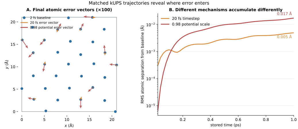
The 2 fs baseline is not an exact solution. The plot measures separation from that reference trajectory, not absolute truth. Its value is causal control: the same initial seed and observation times isolate the changed timestep or potential.
The altered potential separates atoms more than the 20 fs map over this 1 ps window, even though its energy span is slightly smaller. That is the atom-level version of the JAX oscillator result: conserving the wrong Hamiltonian can look numerically cleaner while producing a less relevant trajectory.
Replicas test conclusions, not pointwise paths
Two velocity seeds should not produce matching coordinates. Chaotic dynamics makes pointwise agreement a poor expectation even when both trajectories are valid. Replicas instead test whether a protocol-level conclusion survives initial-state variation.
For the full 2 fs float32 runs, maximum energy excursions range from 0.528% to 0.545%. The float64 result at 0.540% sits inside that range. On this metric and time window, changing precision does not exceed ordinary replica variation. That statement is narrower than “float32 is accurate.” A longer run or a different observable may resolve another effect.
Build an error audit in the right order
Use controls that isolate one mechanism:
- Test the update against an exact or high-accuracy reference problem.
- Sweep timesteps at fixed initial state, duration, and storage cadence.
- Compare deployed precision policies on the target hardware.
- Repeat independent seeds before treating one envelope as typical.
- Check that reported energies and propagated forces are differentiably consistent.
- Validate energy and force predictions against an external reference.
- Repeat the convergence study for the observable supporting the scientific claim.
The final step prevents a common shortcut. A timestep acceptable for mean potential energy need not resolve a vibrational spectrum, diffusion coefficient, or rare-event rate.
Check your understanding
Before changing the notebook, predict each outcome:
- Halve the timestep while doubling the number of steps so final time remains fixed. Which error should decrease first?
- Keep the weak force but switch the measured energy between \(U\) and \(0.98U\). Which energy trace is flatter, and why is the trajectory unchanged?
- Change only the velocity key. Should matched-atom RMS separation remain a useful error metric?
- Replace the artificial quantizer with float32 arrays. What additional hardware and reduction-order evidence would you record?
The second prediction separates dynamics from diagnosis. The same propagated states can appear inconsistent or conservative depending on which Hamiltonian is measured.
Error claims need a named mechanism and observable
Post 02 showed that an integrator defines a discrete path. This chapter adds three more facts: arithmetic perturbs that path, a potential selects the vector field, and initial states create legitimate variation. No single energy number identifies all three.
A defensible result states what changed, what stayed fixed, which observable was compared, and which reference supports the conclusion. That is the error contract the remaining chapters will use for thermostats, barostats, sampling, and learned potentials.
Reproducibility record and complete diagnostic dashboard
Run and verify the CPU profile from a locked environment:
git clone https://github.com/sungsoo-ahn/kups-md-tutorials
cd kups-md-tutorials
uv sync --locked

uv run kups-tutorial run 03 --profile smoke
uv run kups-tutorial verify 03 --profile smoke
uv run kups-tutorial verify-notebooks --posts 03 --output-dir notebook-runs
uv run kups-tutorial export-notebook-cells \
  --executed-notebooks-dir notebook-runs \
  --site-root ../sungsoo-ahn.github.io --posts 03 --check
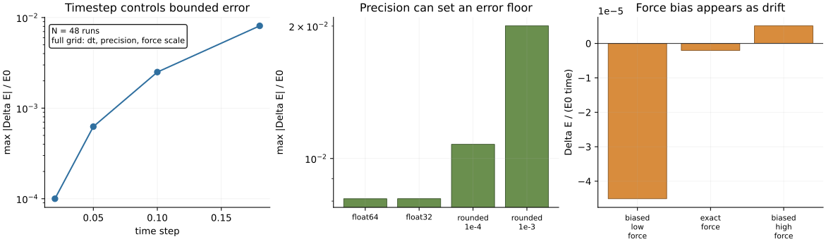
The complete four-panel audit retains the analytic timestep sweep, artificial rounding cases, force-consistency control, energy traces, drift fits, and replica comparisons:
Source and evidence: