An MD integrator turns an instantaneous force into a trajectory. It does not solve Newton’s equations continuously. It constructs a finite-timestep map, and the details of that map determine whether the numerical motion is stable, reversible, and accurate enough for the observable we want.
Velocity Verlet is a useful first integrator because its entire implementation fits in a few JAX lines. We will derive those lines, run them on a harmonic oscillator with an exact solution, locate the same operations inside kUPS, and then watch atoms move in a recorded kUPS trajectory (Verlet, 1967).
- why a timestep creates a numerical trajectory rather than an exact one;
- how half kick, drift, force evaluation, and half kick become JAX operations;
- why velocity Verlet evaluates the force at the new position;
- how kUPS composes the same operations into a production propagator;
- how to compare timesteps without changing the simulated duration or output cadence.
Prerequisites: the MD state, force as a negative energy gradient, and JAX PyTrees from the foundations lesson. Post 01 supplies the controlled many-atom initial state used here.
Continuous equations do not specify a computer update
For atom \(i\) with position \(\mathbf{r}_i\), momentum \(\mathbf{p}_i\), mass \(m_i\), and force \(\mathbf{F}_i\), Newton’s equations are
\[\frac{d\mathbf{r}_i}{dt}=\frac{\mathbf{p}_i}{m_i}, \qquad \frac{d\mathbf{p}_i}{dt}=\mathbf{F}_i(\mathbf{R}).\]The force depends on the positions of all atoms, collected in \(\mathbf{R}\). These differential equations describe the slope of the exact trajectory at each instant. A simulation must choose how to move a finite time \(\Delta t\).
Write the complete state at step \(n\) as \(X_n\). An integrator defines a map
\[X_{n+1}=\Phi_{\Delta t}(X_n).\]Two programs can use the same potential and the same initial state but produce different trajectories if their maps differ. The string verlet is therefore not enough evidence. We need to know which quantities are stored at integer steps, where the forces are evaluated, and how boundaries are applied.
Velocity Verlet is kick, drift, force, kick
Velocity Verlet splits one step into four operations. First, the old force changes the momentum for half a timestep:
\[\mathbf{p}_{n+1/2} =\mathbf{p}_n+\frac{\Delta t}{2}\mathbf{F}(\mathbf{R}_n).\]Second, that half-step momentum moves the positions for a full timestep:
\[\mathbf{R}_{n+1} =\mathbf{R}_n+\Delta t\,\frac{\mathbf{p}_{n+1/2}}{\mathbf{m}}.\]Division by \(\mathbf{m}\) acts atom by atom. Each scalar mass is broadcast across its three Cartesian momentum components. Periodic simulations wrap this position update through the cell.
Third, the potential is differentiated at the new positions:
\[\mathbf{F}_{n+1}=-\nabla_{\mathbf{R}}U(\mathbf{R}_{n+1}).\]Finally, the new force completes the second half kick:
\[\mathbf{p}_{n+1} =\mathbf{p}_{n+1/2}+\frac{\Delta t}{2}\mathbf{F}_{n+1}.\]Reusing \(\mathbf{F}(\mathbf{R}_n)\) in the last line would define a different method. The program might still advance atoms and produce a smooth movie, but it would no longer implement velocity Verlet.
The equations translate directly into JAX
The notebook setup imports a minimal ParticleState containing positions, momenta, and masses. It also imports the types needed by the displayed function. Setup and paths are collapsed because they do not define the algorithm.
Python
from functools import partial
from pathlib import Path
import os

repo_root = Path.cwd()
if not (repo_root / "configs").exists():
    repo_root = repo_root.parent
os.chdir(repo_root)
os.environ.setdefault("JAX_PLATFORMS", "cpu")

from IPython.display import Image, display
import jax
import jax.numpy as jnp
from kups_md_tutorials.jax_reference import EnergyFunction, ParticleState
from kups_md_tutorials.kups_engine import (
    load_kups_md_experiment,
    run_kups_md_experiment,
)
The next cell is the complete tested reference step. Each assignment matches one equation above.
Python
def velocity_verlet_step(
    energy_fn: EnergyFunction,
    state: ParticleState,
    time_step: float,
) -> ParticleState:
    """Advance one velocity-Verlet step using autodifferentiated forces."""

    forces = -jax.grad(energy_fn)(state.positions)
    half_momenta = state.momenta + 0.5 * time_step * forces
    positions = state.positions + time_step * half_momenta / state.masses[:, None]
    next_forces = -jax.grad(energy_fn)(positions)
    momenta = half_momenta + 0.5 * time_step * next_forces
    return ParticleState(positions, momenta, state.masses)


def oscillator_energy(positions):
    return 0.5 * jnp.sum(positions**2)


state = ParticleState(
    positions=jnp.array([[1.0, 0.0, 0.0]]),
    momenta=jnp.zeros((1, 3)),
    masses=jnp.ones(1),
)
step = jax.jit(partial(velocity_verlet_step, oscillator_energy, time_step=0.2))
next_state = step(state)
print(f"q: {state.positions[0, 0]:.3f} -> {next_state.positions[0, 0]:.3f}")
print(f"p: {state.momenta[0, 0]:.3f} -> {next_state.momenta[0, 0]:.3f}")q: 1.000 -> 0.980
p: 0.000 -> -0.198
The one-dimensional oscillator begins at \(q=1\) with zero momentum. For \(\Delta t=0.2\), the first force is \(-1\). The half kick gives \(p_{1/2}=-0.1\), the drift gives \(q_1=0.98\), and the second force is \(-0.98\). The final momentum is therefore \(p_1=-0.198\), exactly matching the output.
Three JAX choices are doing useful work here:
-
jax.grad(energy_fn)constructs the force calculation from the scalar potential energy. - The function returns a new
ParticleState; it does not mutate the input. -
jax.jitcompiles the step for the state shapes and selected device.
A trajectory applies this compiled step repeatedly with jax.lax.scan. The foundations notebook showed that loop. Keeping the step and loop separate makes the numerical map inspectable without giving up compiled execution.
The first force in a long trajectory does not need to be recomputed twice per step. A production engine can cache \(\mathbf{F}_n\) from the previous step, perform the first half kick, and evaluate the potential once at \(\mathbf{R}_{n+1}\). The reference function evaluates both forces because its input deliberately contains only the three essential state arrays.
An exact oscillator isolates integration error
For a unit harmonic oscillator,
\[\ddot q=-q, \qquad q(t)=q(0)\cos t+v(0)\sin t,\]so the numerical position can be compared with an exact value at every step. Its energy is
\[E=\frac{1}{2}v^2+\frac{1}{2}q^2.\]This control removes neighbor lists, periodic boundaries, cutoffs, and force-field uncertainty. Any observed error comes from the finite-timestep map and floating-point arithmetic.
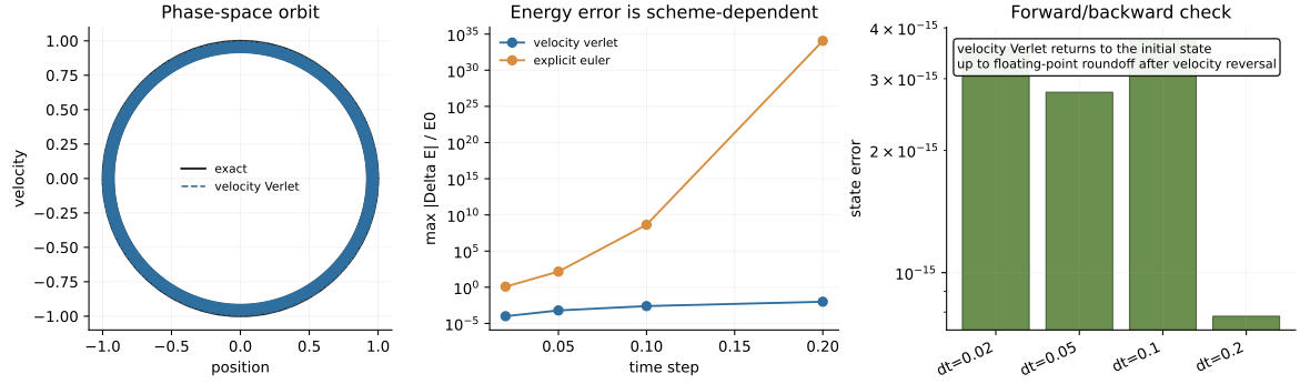
At \(\Delta t=0.2\), the committed 2,000-step control has a maximum relative energy error of approximately 1%. Its forward/reverse state error is below \(10^{-15}\) in float64. Across timesteps 0.02, 0.05, 0.1, and 0.2, the maximum energy error grows from \(10^{-4}\) to \(10^{-2}\).
Velocity Verlet is time reversible for this deterministic system: integrate forward, reverse momentum, apply the same map again, and the state returns to its starting point up to roundoff. Explicit Euler fails this structural test and expands the phase-space orbit.
Reversibility does not imply an exact path or exactly constant reported energy. A stable symplectic method commonly follows a nearby shadow Hamiltonian, so the physical energy oscillates within a bounded envelope instead of drifting monotonically (Hairer et al., 2006). The envelope still widens as the timestep grows.
kUPS composes the same four operations
kUPS adds the machinery omitted from the reference function: indexed particle and system tables, periodic flows, cached potential derivatives, step counters, error handling, block execution, and HDF5 logging.
For the verlet integrator, kUPS 1.0.3 constructs a sequential propagator with this order:
-
MomentumStepwith \(\Delta t/2\); -
PositionStepwith \(\Delta t\) and the configured boundary flow; - the potential derivative propagator at the new state;
-
MomentumStepwith \(\Delta t/2\).
That is the same kick–drift–force–kick map as the reference JAX function. kUPS stores position gradients and exposes forces with the corresponding negative sign, while its potential cache avoids unnecessary evaluations.
The next cell runs the public library path on Lennard-Jones argon. Both CPU smoke cases begin from the same seeded positions and momenta. Only the timestep changes.
Python
kups_spec = load_kups_md_experiment("02", "smoke")
kups_result = run_kups_md_experiment(
    kups_spec,
    raw_run_dir=Path("runs/notebook-post-02/smoke"),
    quiet=True,
)
for case in kups_result.cases:
    print(
        f"{case.name}: frames={case.frame_count}, atoms={case.atom_count}, "
        f"max |dE/E0|={case.max_abs_relative_energy_error:.3e}, "
        f"device={case.observed_devices[0]}, hdf5={case.hdf5_sha256[:12]}"
)verlet_dt_0_5fs: frames=8, atoms=32, max |dE/E0|=9.104e-07, device=cpu:cpu, hdf5=8db7f88f86c9
verlet_dt_20_0fs: frames=8, atoms=32, max |dE/E0|=2.588e-03, device=cpu:cpu, hdf5=cbca97ecad50
This output establishes more than a successful import. kUPS advanced 32 atoms, wrote eight frames per case, reopened the HDF5 files, and measured their energy error. The hashes identify the exact raw trajectories used by the verification step.
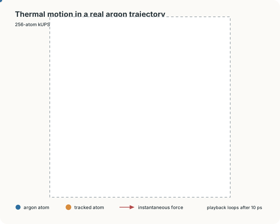
The animation is a projection of recorded coordinates, not an artist’s impression. It selects the 32 atoms closest to the initial \(z=0\) lattice layer from the 2 fs full-profile HDF5 trajectory. Atoms near a dashed edge have periodic neighbors on the opposite edge. The selected identities remain fixed even when an atom moves slightly out of the initial plane.
A timestep comparison must hold physical time fixed
Comparing 500 steps at several timesteps would compare different simulated durations. Comparing every integration step would also change the output cadence. The full experiment instead holds both the duration and stored-frame spacing fixed at 10 ps and 20 fs:
| Timestep | Integration steps | Stored frames | Max stored-frame \(\lvert\Delta E/E_0\rvert\) | Energy span |
|---|---|---|---|---|
| 0.5 fs | 20,000 | 500 | 0.528% | 0.383 meV/atom |
| 2 fs | 5,000 | 500 | 0.528% | 0.383 meV/atom |
| 20 fs | 500 | 500 | 0.633% | 0.459 meV/atom |
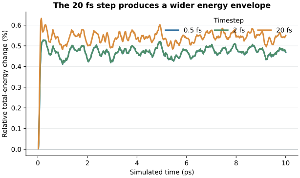
This result does not establish 2 fs as a universal choice. The fastest relevant motion sets the useful scale. A bonded hydrogen vibration, a stiff constraint, a close collision, and a smooth argon crystal can require different timesteps. A machine-learned potential can also introduce steep or noisy regions absent from its training data.
The experiment supports a narrower conclusion: for this initialized argon crystal and this 10 ps window, reducing the step from 2 fs to 0.5 fs does not change the stored energy trace visibly, while increasing it to 20 fs widens the envelope.
Stable energy is necessary but not sufficient
A sloping energy trace can indicate a timestep that is too large. It can also come from a discontinuous cutoff, a stale neighbor list, insufficient precision, loose constraints, or forces inconsistent with the reported energy.
The converse is also true. Bounded energy does not prove that each atomic position is accurate over long times. Chaotic trajectories separate even when their ensemble statistics remain useful. Choose a timestep against the observable you intend to estimate, not against visual smoothness alone.
A practical diagnostic sequence is:
- Test the update on a system with an exact solution.
- Confirm reversibility or another structural property when the method should have it.
- Sweep timesteps on the real potential and initial state.
- Hold duration and output cadence fixed.
- Inspect both bounded fluctuations and systematic drift.
- Repeat after changing precision, neighbor policy, constraints, or the force model.
Post 03 separates these error sources. Reducing \(\Delta t\) can reduce discretization error, but it cannot repair a systematically wrong or non-conservative force.
Check your understanding
Suppose the second jax.grad call in the displayed JAX step is deleted and the old force is reused for the final half kick. Predict which test will expose the change first: a one-step position check, a one-step momentum check, or a long energy trace.
The one-step position is unchanged because the drift already used the first half-step momentum. The one-step final momentum changes immediately because it should use the force at the new position. The long energy trace then amplifies that local mistake. A useful unit test should therefore compare the momentum after one known step rather than waiting for a simulation to become unstable.
Reproducibility record and full diagnostic dashboard
The full manifests record an observed NVIDIA RTX A5000 backend for every production case. The CPU smoke results establish portable execution; the GPU results support the 10 ps quantitative comparison. The animation provenance records the HDF5 SHA-256 hash, dataset names, displayed frame indices, selected atom identities, projection, wrapping convention, and force-vector scale.
git clone https://github.com/sungsoo-ahn/kups-md-tutorials
cd kups-md-tutorials
uv sync --locked

uv run kups-tutorial run 02 --profile smoke
uv run kups-tutorial verify 02 --profile smoke
uv run kups-tutorial verify-notebooks --posts 02 --output-dir notebook-runs
uv run kups-tutorial export-notebook-cells \
  --executed-notebooks-dir notebook-runs \
  --site-root ../sungsoo-ahn.github.io --posts 02 --check
The repository contains the smoke configuration, full configuration, CPU summary, GPU summary, full provenance manifest, notebook, figure source, and review record.